Maximize Data Lookup Efficiency with Google Sheets MATCH Function

The MATCH function in Google Sheets can improve your performance if you need to search for a specific value within a range, especially when dealing with large datasets. Using the MATCH function allows you to efficiently locate the position of a value within a dataset, making it easier to analyze and manage structured collections of data.

In this article, we’ll explore the ways you can use the MATCH function in Google Sheets; see how it can make your work easier, how you can combine it with other functions; and we’ll tackle some common issues you might run into when using it.

Basics Of The MATCH Function in Google Sheets For Dynamic Data Searches

The MATCH function is similar to a search engine for the data in a one-dimensional array in Google Sheets. You give it a value to look for, and it tells you the relative position of that value in a selected range of cells.

Here’s why you might need to use MATCH in Google Sheets:

• Find the position of an item. Instead of manually searching through the entire column, MATCH can quickly locate the position of that value, returning the exact match position of the value within the cell range.‍
• Index-Match combination. When combined with the INDEX function, MATCH can dynamically retrieve values from a dataset based on certain criteria, by finding the exact position in a lookup column or specified column. This combination is much faster and more efficient than using VLOOKUP or XLOOKUP functions.

MATCH Function Syntax

The syntax of the MATCH function is the following:

=MATCH(search_key, range, [search_type])

Where:

• search_key: The specified value you are searching for.
• range: The range of cells where you want to search for the search_key.
• [search_type]: (Optional) Sets the type of match:some text
  • 1 for less than or equal to (returns the largest value less than or equal to the search_key).
  • 0 for an exact match.
  • -1 for greater than or equal to (returns the smallest value greater than or equal to the search_key).
  • If omitted, the default is 1 (less than or equal to).
    

MATCH Formula Practical Application in Google Sheets

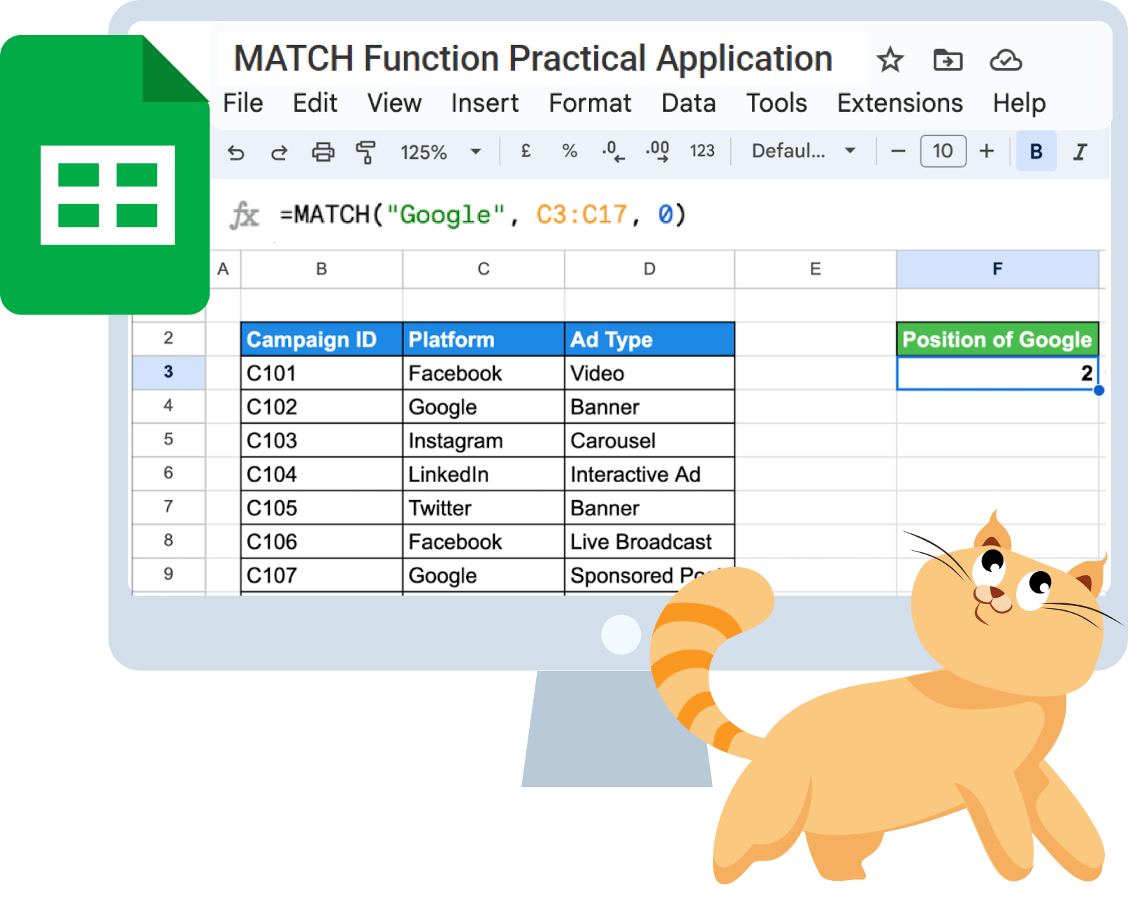
Let's break down the syntax of the MATCH function using an example with campaign IDs and platforms.

Our task is to find the position of the campaign with the platform "Google" in the list.

Our table's range is B3:D17, and we want to search within the Platform column (Column D).

Here's how we can use the MATCH function:

=MATCH("Google", C3:C17, 0)

Now, let's analyze the formula:

• search_key: This is the value we are searching for. In our case, the value is "Google" within the Platform (C) column.
• range: This is the range, within which we are searching, specifically C3 to C17.
• [search_type]: If this parameter is set to 0, the MATCH function will only return a result if it finds the exact value. If there's no exact match, it will return an error (#N/A).

After entering the MATCH formula, Google Sheets returns the position number 2. This means that within the range C3:C17 (the "Platform" column), "Google" is found in the second position, counting from the top row. Essentially, the MATCH formula returns the relative position of “Google” within the specified range.

Grab Your Essential MATCH Function Template Now!

Tap into the power of dynamic data retrieval with our MATCH function template. Every tutorial and example from our article is pre-set for you to understand and implement the MATCH function effectively. Just download, open, and start enhancing your data analysis skills instantly.

Download your FREE template today!

Key Differences Between MATCH and VLOOKUP in Google Sheets

The core distinction between the two functions, MATCH and VLOOKUP, lies in their output and lookup direction. The MATCH function returns the position of a value within a single row or column. In contrast, VLOOKUP searches for a value in the first column of a range and returns a corresponding value from a specified column in the same row.

Common Examples Of Using The MATCH Function In Different Scenarios

We’d like to share some common examples where you might find the MATCH function useful. The MATCH function can be used in various scenarios for data lookup and matching.

MATCH Function In A Sorted Range

Now, let's say we want to find the position of the ad type "Banner" within this sorted range.

Here's how we can use the MATCH function:

=MATCH("Banner", B3:B17, 0)

When we input this formula into a cell, it will return the position of the first occurrence of "Banner" within the sorted range of ad types.

MATCH Function With Text String As Search Key

Similarly to the previous example, we can search for a specific text string within a range of data, whether sorted or not, using the MATCH formula for an exact match. Let's find the position of the ad type "Live Broadcast"

The MATCH function will be the same:

=MATCH("Live Broadcast", B3:B17, 0)

MATCH Function With A Dynamic Lookup Value

Now, we want to find the position of a dynamically changing ad type. Let's use a cell reference containing the ad type we want to search for.

Suppose the ad type we're interested in is entered in cell D3. Let's use the MATCH formula to find its relative position.

Here's the formula:

=MATCH(D3, B3:B17, 0)

Google Sheets will search for the ad type that is mentioned in cell D3. If the ad type in D3 is "Sponsored Post" and it appears in row 6, the formula will return 4.

MATCH Function In A Horizontal Range

To find the relative position of the ad type "Banner" within the horizontal range, we can use the following MATCH formula:

=MATCH("Banner", B2:E2, 0)

Where:

• "Banner": This is the ad type we're searching for.
• B2:E2: This is the horizontal range where we're searching for the ad type.

If you need to work with horizontal ranges, the UNIQUE function in Google Sheets can be incredibly useful, as it automatically identifies and returns the unique values found in the horizontal range. For more detailed usage of the UNIQUE function, you can read our guide.

MATCH Function With An Approximate Match

To find an approximate match of campaign costs using the MATCH function, first ensure that the Campaign Costs are sorted in ascending order. Then, we can use the MATCH function with the third argument set to 1 to find the relative position of the largest value less than or equal to the lookup value.

The Campaign Costs are listed in cells B3:B17. Suppose we want to find the approximate match of the campaign cost of 200.

Here's how you can use the MATCH function with an approximate match:

=MATCH(200, B3:B17, 1)

Where:

• 200: This is the value we're searching for, which represents the campaign cost we want to find.
• B2:B17: This is the range where we're searching for the campaign costs.
• 1: We use 1 for an approximate match because we want to find the position of the largest value less than or equal to 200.

MATCH Function With Date As Search Key

Now, let's say we want to find the position of the date 21 May 2024 (or 21/05/2024) within this range using an exact match to avoid mismatches with similar dates.

Here's how you can use the MATCH function:

=MATCH(DATE(2024, 5, 21), B3:B17, 0)

Where:

• DATE(2024, 5, 21): This constructs the date "21/05/2024" using the DATE function.
• B3:B17: This is the range where we're searching for the date.

How to Extract Data Using MATCH with Other Google Sheets Functions

The MATCH formula can be combined with other functions, such as INDEX, VLOOKUP, and IFERROR, to perform more complex tasks in Google Sheets.

Let’s take a closer look at how each combination works:

MATCH Formula With INDEX (Index Match) In Google Sheets

When combined INDEX and MATCH functions can dynamically retrieve values by using MATCH to find the position and INDEX to return the corresponding value.

Using the INDEX MATCH function in Google allows for more flexible data lookups, especially when you need to satisfy all the criteria in complex lookups by combining these functions. 

Additionally, INDEX MATCH can handle bi-dimensional arrays, allowing for more versatile data retrieval, making it a preferred choice for complex datasets.

For example, with a list of campaign IDs in column B and corresponding ad types in column C, we can use MATCH to find the relative position of a specific campaign ID in the lookup column (in this case, column B), and then use Google Sheets INDEX function to retrieve the corresponding ad type from column C. 

Use this formula for INDEX MATCH:

=INDEX(C:C, MATCH("C102", B:B, 0))

Using MATCH With VLOOKUP for Case-Sensitive Vertical Lookup

In Google Sheets, the MATCH can be effectively combined with VLOOKUP to perform dynamic vertical lookups. This method is especially useful when you need to retrieve data based on variable column positions that are not fixed, while still ensuring an exact match.

Suppose you have a dataset containing campaign IDs and their corresponding costs in a table. You want to look up the cost of a campaign based on its ID, where the ID and the cost columns may vary in their position within the table.

To achieve this, you can use the MATCH function to dynamically find the column index of the campaign cost and then use VLOOKUP to fetch the cost for a specific campaign ID.

Use the formula:

=VLOOKUP(G2, B3:D, MATCH(G3, B2:D2, 0), FALSE)

In this example:

• G2: This cell should contain the campaign ID you’re searching for.
• B3:D: The range that includes campaign IDs and their respective costs.
• MATCH(G3, B2:D2, 0): This formula finds the column index of the campaign cost dynamically by searching for the header (assumed to be in cell G3) in the header range B2:D2. This identifies the specified column from which the data related to the specified value will be retrieved.
• VLOOKUP then searches for the campaign ID in the specified range and returns the cost from the specified column at the row found for the campaign ID.

This approach allows the formula to adapt to changes in the column order across different sheets without any manual adjustment, enhancing its flexibility and reliability in dynamic datasets.

💡If manual processes are causing you headaches, consider using tools that automate data retrieval and overcome the limitations of the standard VLOOKUP formula with IF statements. Explore our complete guide on using VLOOKUP with IF statements in spreadsheets to simplify and enhance your data handling tasks.

MATCH Function With IFERROR

If MATCH doesn't find a match, it returns an error. You can combine IFERROR with MATCH to handle errors gracefully.

If we're using MATCH to find the position of a value in a range, we can wrap the MATCH function with IFERROR to display a custom message or value instead of the error if no match is found.

Use the formula:

=IFERROR(MATCH("Poll", C2:C17, 0), "Not found")

Troubleshooting Common Errors With The MATCH Function

Even if you use Google Sheets' Match Function formulas daily, mistakes can still happen. Here are some common errors to look out for and how to fix them quickly:

Resolving #N/A Error

This error occurs when the value you are looking for is different from the ones within the range. Check if the data or reference exists, and ensure it's correctly spelled or formatted. If it's a formula error, verify the logic and input values. Additionally, the #VALUE! An error occurs due to incorrect data types in the MATCH function's parameters, so ensure that the data types match the expected input.

Fixing #VALUE! Error

This error tells about an incorrect data type or operation. For example, you can mistakenly use 01/15/2023 as a text-formatted date instead of a date value. In this case, verify that the data is in the correct format (convert it if necessary) and adjust the formula accordingly.

Correcting #REF! Error

The #REF! error means there's a problem with a cell reference. Verify the cells referenced in your formula and update them as needed. Make sure you didn't delete or move any cells that the formula is using. If you did, adjust the formula to include the correct cells.

Clarifying #NAME? Error

This error means the formula doesn't recognize a function or named range. Check the spelling and how it's written in the formula. Make sure all functions and ranges are named correctly and used properly.

Mitigating #NUM! Error

This occurs when a mathematical calculation fails, for example, dividing by zero or using negative numbers. Adjust the formula to handle these situations correctly or use the right numbers for calculations.

While spreadsheets help manage and organize data, not everyone on your team may be familiar with them. It's a good idea to use tools that can help you better organize, manage, and analyze your data beyond spreadsheets.

MATCH Function Best Practices For Optimal Performance

Here are some best practices you can use to maximize its efficiency when using the Google Sheets MATCH function to search for a specific value within a designated range in Google Sheets:

Understanding MATCH Types

Learn the differences between exact match (0), close match (1), and reverse close match (-1) in MATCH to ensure the correct lookup type is applied.

Using Named Ranges

Name ranges in your sheet to simplify formulas. This makes formulas easier to understand and manage, especially in big or complicated sheets.

Update And Maintain Your Data

Regularly check your data in Google Sheets for mistakes. Keep it accurate and consistent so that MATCH works correctly and provides the right results.

Use Comments And Documentation

By providing clear explanations alongside your MATCH functions, you make it easier for anyone reviewing the sheet to grasp how data is imported and manipulated. This practice helps others, including your future self, to better understand your work.

Improve Your Google Sheets Skills With These Guides

If you want to improve your Google Sheets skills, learn more about mastering functions like the Index Match formula and other advanced functions like ARRAY, Pivot Table, etc.

• ARRAY: Conducts calculations across multiple cells or ranges, delivering multiple results simultaneously.
• Pivot Table: This adaptable tool simplifies the summarization, organization, and examination of extensive data sets, allowing for easy extraction of insights and identification of trends.
• CONCATENATE Function: This function combines multiple text items into a single continuous string, providing a seamless way to merge text from different cells.
• FILTER Function: This function in Google Sheets is used to extract data that meets certain criteria from a range of cells.
• SEARCH function: It is used to locate the position of a substring within a string, without considering case sensitivity.

For a step-by-step guide on using the INDEX and MATCH functions in Google Sheets, check out our detailed blog post.

Elevate Your Google Sheets Data Analysis With OWOX: Reports, Charts & Pivots Extension

With the OWOX: Reports, Charts & Pivots Extension, you can easily pull data from BigQuery directly into Google Sheets to create comprehensive reports. The extension allows you to build dynamic charts, generate pivot tables, apply filters, and aggregate data in real-time. It ensures live data updates and simplifies sharing up-to-date reports, charts, and pivots with your team.