Using the SEARCH Function in Google Sheets: From Basics to Advanced Techniques

Let’s find out how to use the SEARCH formula in Google Sheets. This search function works well for finding the location of a certain word or combination of letters in text strings. Opening a Google Sheets document is essential as a starting point for using the SEARCH function.

Additionally, the Google Sheets SEARCH function can determine whether a word is contained in a text. This article will provide general information, examples, and suggestions for use.

Note: This article was originally published in June 2024, and completely updated in January 2025 to ensure accuracy and comprehensiveness regarding the SEARCH function in Google Sheets.

What is the SEARCH Function in Google Sheets?

The SEARCH formula returns a whole number indicating the position at which a particular string is first found within a specific text.

It is handy for pinpointing the exact spot of a word or a combination of letters. Even if you just need to check if a word is present, this function can be a great tool. Notice, that it is not case-sensitive. For case-sensitive searches, use the FIND formula instead. The SEARCH function helps you locate a specific substring within a text string, making it easier to understand its inputs and how it works.

Exploring the Basics of the SEARCH Function

The SEARCH function in Google Sheets helps you find the position of a specific string of characters, or the substring, within a larger text.

A key feature of the SEARCH function is its ability to start the search from a specified position within the text. By default, it starts at the first character, but you can set it to begin at any character position. This is particularly useful when dealing with large texts where you want to skip certain sections. To manage large datasets efficiently, it is crucial to search effectively by using it correctly.

Follow these steps to use the SEARCH function in Google Sheets:

1. Type "=SEARCH" or go to "Insert" → "Function" → "Text" → "SEARCH". You can also navigate directly to the "Functions" icon.
2. Specify a string you want to look up and text where the formula searches the specified string. If necessary, input at which the search starts (e.g., starting the search from the third letter in the selected text).
3. Press the "Enter" key.

SEARCH Function Syntax

The SEARCH function in Google Sheets has a simple syntax:

=SEARCH(search_for, text_to_search, [starting_at])

Let's break down what these parameters represent:

• search_for: the substring to look for within the text.
• text_to_search: the main text string within which to look for the first occurrence of the search_for substring.
• starting_at (optional): the position in text_to_search from which the function starts to search.

As covered in the syntax, the SEARCH function requires both the string and the substring. The third parameter, [starting_at], is optional. You only need to use this if there are multiple occurrences of the same substring.

SEARCH Function Examples

The list of examples will help you gain a better understanding of the SEARCH function by demonstrating its practical applications. Seeing the function in action can clarify how it works and reveal the nuances of its usage.

By working through these examples, you'll learn how to handle different scenarios, such as partial matches and wildcard searches. Ultimately, examples provide a straightforward and effective way to master the SEARCH function in Google Sheets.

Get Your Spreadsheet Work Done with Our SEARCH Template!

Watching the function in action clarifies its workings and highlights its nuances, while working through examples teaches you to handle scenarios, making it an effective way to master the SEARCH function in Google Sheets.

Download your FREE template today!

Practical Examples of the SEARCH Function in Google Sheets

Here, we've put together the 5 most common ways to use the SEARCH function in Google Sheets. These examples will cover the most common usage cases and help you follow the syntax rules.

Example #1: Locating a Specific Word within Text with SEARCH

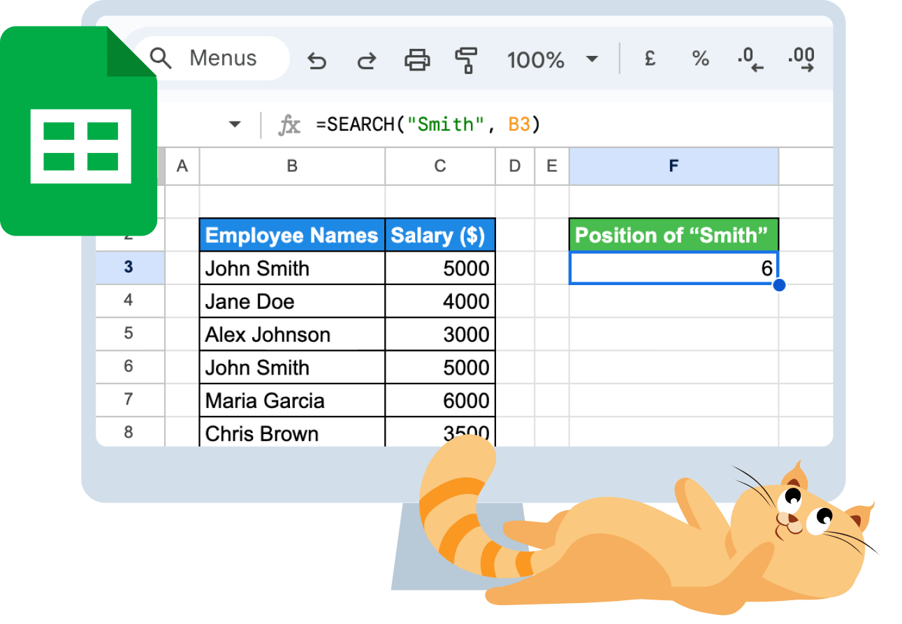
Suppose you have a cell B3 with the text “John Smith” and want to find the position of the word “Smith”.

You can use the SEARCH function as follows:

=SEARCH("Smith", B3)

The function will return 6, the position of the first letter of the word “Smith” in the text string.

Example #2: SEARCH without Case Sensitivity

The SEARCH function is not case-insensitive. This means it treats lowercase and uppercase characters as the same. Suppose you have a cell B5 with the text “Alex Johnson” and want to find the position of the word “Alex”.

You can use the SEARCH function as follows, without noticing whether it starts with a lowercase or capital letter:

=SEARCH("alex", B5)

The function will return 1, which is the position of the first letter of the word “Alex” in the text string.

Example #3: Employing Wildcards in SEARCH

The SEARCH function supports wildcard characters, which can be helpful when you're unsure of the exact word or phrase you're looking for. For instance, in the list of employees, if cell A1 contains the text "Maria Garcia" and you want to find the position of a last name that starts with "g" and ends with "a", you can use the SEARCH function as follows:

=SEARCH("g*a", B7)

The function will return 7, which is the position of the first letter of the word “Garcia” in the text string of the B7 cell.

Example #4: Finding the Position of a Particular Character with SEARCH

You can also use the SEARCH function to find the position of a specific character in a text string. For instance, if you have a cell B7 with the text “Maria Garcia” and you want to find the position of the “c” character, you can use the SEARCH function as follows:

=SEARCH("c", B7)

The function will return 10, which is the position of the "c" letter of the word “Garcia” in the B7 text string.

Example #5: Conducting Searches Starting at a Designated Position with SEARCH

The SEARCH function also allows you to specify a starting position for the search. For example, if you have a cell B7 with the text “Maria Garcia” and you want to find the position of the second occurrence of the letter “a”, you can use the SEARCH function as follows:

=SEARCH("a", B7, 3)

The function will return 5, which is the position of the second occurrence of the letter 'a' in the B7 text string 'Maria Garcia', starting from the third letter.

Make sense of your data

Automatically generate Pivots & Charts in Google Sheets!

Visualize Your Data

Leveraging SEARCH with Other Google Sheets Functions

The SEARCH function in Google Sheets is versatile on its own, but it becomes even more powerful when combined with other functions. When learning how to search in Google Sheets effectively, integrating SEARCH with functions like VLOOKUP, IFERROR, ISNUMBER, LEN, and MID, you can perform more complex text manipulations and analyses. The Google Sheets search function is effective for finding substrings within text strings, allowing users to locate specific text efficiently.

These combinations allow you to handle errors, validate text, and extract specific parts of text. In the following examples, you'll see how to leverage the SEARCH function alongside other functions to enhance your spreadsheet capabilities.

Combining SEARCH with IFERROR Function

The IFERROR function acts as a safety net when paired with SEARCH, ensuring smooth operations even if the SEARCH function encounters errors. If you're exploring how to search in Google Sheets effectively using IFERROR, you can specify a value to return when the SEARCH function fails to find the desired string.

This capability is especially handy when searching for a string that may not exist in every cell of the dataset. In such cases, IFERROR helps prevent formula errors and ensures consistent results throughout your analysis. Combining IFERROR with SEARCH enhances the reliability and robustness of your spreadsheet functions.

Here's the general syntax of the IFERROR function:

=IFERROR(value, [value_if_error])

Let's clarify the meaning of these parameters:

• value: the formula or expression to evaluate.
• [value_if_error]: the value to return if the formula or expression results in an error. This argument is optional; if omitted, IFERROR will return a blank cell when an error is encountered.

Assuming we have a list of employees in column B, and we want to find out if Chris Brown is listed.

=IFERROR(SEARCH("Chris Brown", B3:B10), "Yes")

We can use the SEARCH function combined with IFERROR to return "Yes" if the name is found.

Merging SEARCH with ISNUMBER Function

The ISNUMBER function evaluates whether the result of the SEARCH function is a number, indicating a successful match. This combination allows for efficient validation of whether a specific string is present within a cell.

Here's the general syntax of the ISNUMBER function, merging with SEARCH:

=ISNUMBER(SEARCH(substring, range))

• substring: the text you are searching for within the larger text string.
• range: the cells range where you are searching for the substring.

Assume we have a column of text data in column B, and we want to determine if the word “John” appears in it. We can use SEARCH in combination with ISNUMBER to return TRUE if “John” is found and FALSE if not.

=ISNUMBER(SEARCH("John", B3:B10))

By employing ISNUMBER with SEARCH, you can automate the process of verifying the existence of desired text within your dataset. This approach enhances the accuracy and reliability of your data analysis tasks.

Instant Data Visualization

Turn your raw data into editable charts and pivots

Visualize Your Data

Using SEARCH in Conjunction with LEN Function

The LEN function can be used with SEARCH to find the length of the text before a specific character or substring. By using SEARCH to locate the position of the character and then LEN to measure it, you can determine how many characters precede the target. This combination is useful for extracting or manipulating specific parts of text. It enhances the precision of text analysis in your spreadsheets.

=LEN(text) - SEARCH(substring, text)

• substring: the text you are searching for within the larger text string.
• text: the cells range where you are searching for the substring.

Suppose you have a cell B7 containing the name "Maria Garcia" and you want to find the length of the text after a specific character, "G".

=LEN(B7) - SEARCH("G", B7)

LEN calculates the total length of the text in B7, which is 12. Then the SEARCH function finds the position of the G in the text, which is 7.

So, the result of this formula is 12-7=5, indicating that there are 5 letters after the specific character "G".

Integrating SEARCH with MID Function

The MID function can be used with SEARCH to extract a substring from a cell, starting at the position where a specific string is found. By combining these functions, you can locate the starting point of a desired substring and then extract a specific number of characters from that position.

Here's the general syntax of the MID function, combined with SEARCH:

=MID(range, SEARCH(substring, range), num_chars)

Let's clarify the meaning of these parameters:

• substring: the text you are searching for within the larger text string.
• range: the cells range where you are searching for the substring.
• num_chars: the number of characters to extract.

Suppose you have a cell range (B3:B10) containing the employee's full names, and you want to extract the last name of each employee.

Here is the formula you can use:

=MID(B3, SEARCH(" ", B3) + 1, LEN(B3))

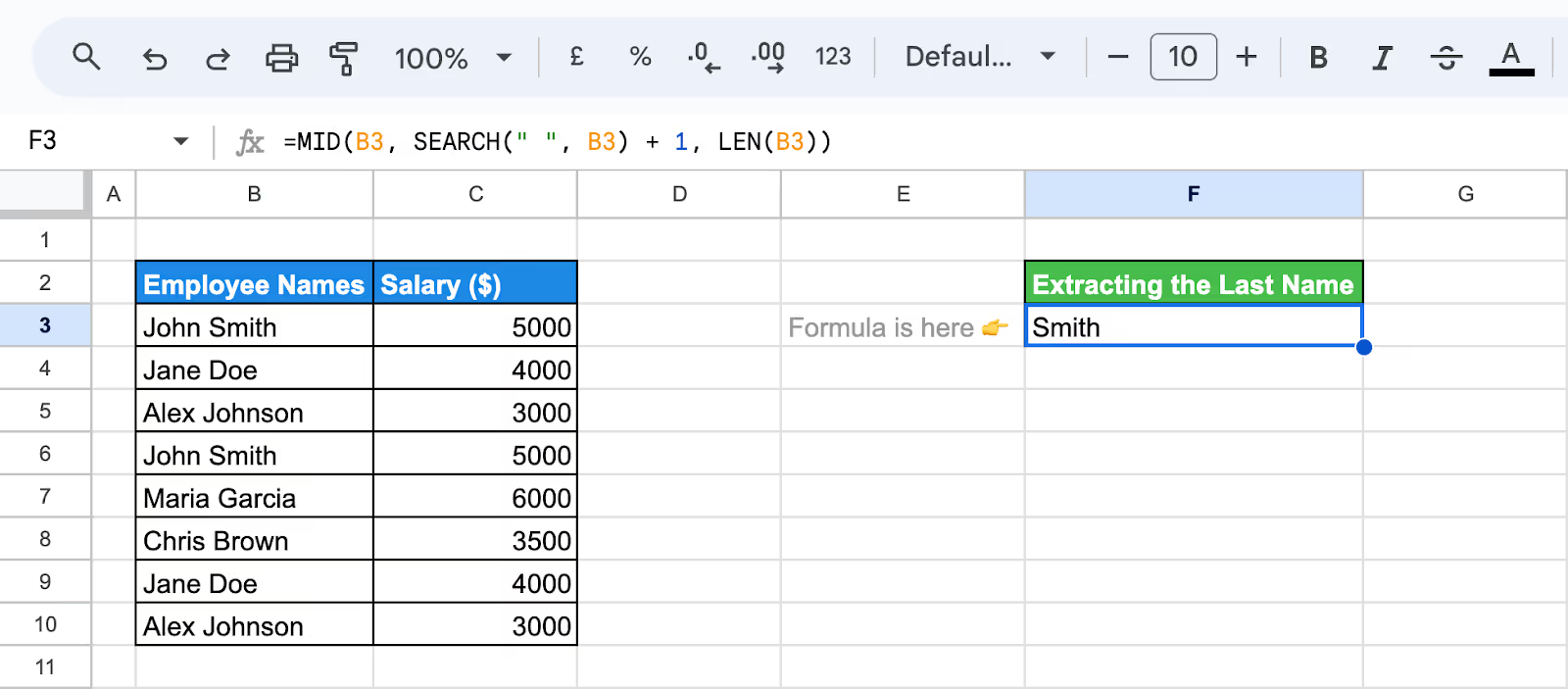
Here is the breakdown:

• SEARCH(" ", B3): This finds the position of the first space in the cell B3.
• + 1: This adjusts the start position to the character right after the space.
• LEN(B3): This ensures that you extract all characters up to the end of the string, starting from the character after the space.

The great thing is that you can easily drag this formula down to extract the last names of all employees in the list, which is perfect if you have a large dataset.

NOTE: If the names are consistently formatted with only one space between the first and last names, this formula will effectively extract the last name. If there's a possibility of multiple names or middle names, this formula will need adjustments to suit the specific format of the names.

Turn Data into Actionable Insights

Auto-generate reports and dashboards from your data in Google Sheets... 100% Free!

Visualize Your Data

SEARCH Function Alternatives in Google Sheets

Manually searching through a large Google Sheets file isn't efficient. Fortunately, a built-in search function can quickly scan all your open documents. Beyond Google's Find function, there are various other ways how to search in Google Sheets to locate information. Here, we will explore each method so you can select the best search technique for your needs.

Using the Find and Replace Feature

While the basic Find feature in Google Sheets serves its purpose well, the platform offers an enhanced tool called Find and Replace, which allows users to specify detailed search criteria for more advanced functionality.

This tool not only locates specific data but also allows users to replace it with new content if desired. With Find and Replace, users can refine their search criteria, specify whether to match cases and even perform batch replacements across the entire spreadsheet.

Follow these steps to use the Find and Replace tool in Google Sheets:

1. Go to "Edit" → "Find and Replace" or press Ctrl + H (Windows) or CMD + Shift + H (Mac).
2. Enter the search term into the Find text box, then click the "Find" button to find your search query.
3. If there are multiple instances of the search query, keep pressing "Find" to look through each instance.
4. When you see the message "No more results found, looping around" on the screen, you are back to the first occurrence of your search query.
5. To restrict the search to the current sheet, select the drop-down menu that says All sheets and change it to This sheet. Alternatively, choose a Specific range to restrict the search to a particular range of cells within the active sheet. If a range is selected, it's defined for you. You can change it by choosing the Select data range option.

Enhancing Search with the VLOOKUP Function

VLOOKUP is a widely used function in Google Sheets for searching and retrieving data from a specified range. VLOOKUP opens up a realm of possibilities for advanced data manipulation and analysis.

Let's quickly review VLOOKUP to simplify your data processing tasks and unlock valuable insights.

The VLOOKUP function in Google Sheets is a powerful tool for searching and retrieving data from a specified range based on a given key. It stands for "Vertical Lookup" and is particularly useful when you have large datasets organized in columns.

Here's the general syntax of the VLOOKUP function:

=VLOOKUP(search_key, range, index, [is_sorted])

Here's what these parameters mean:

• search_key: This is the value you want to search for in the first column of the specified range.
• range: This is the range of cells containing the data you want to search. The first column of this range should contain the search key, and the data you want to retrieve should be in subsequent columns.
• index: This specifies which column within the range contains the data you want to retrieve.
• [is_sorted]: This is an optional parameter that indicates whether the data in the first column of the range is sorted in ascending order. Use TRUE for sorted data (default) or FALSE for unsorted data.

Suppose you have a list of employees' names in column B and their corresponding salaries in column C. You want to find the salary of an employee named "Chris Brown".

Assuming your data starts from cell B3 and ends at cell C10, this formula will search for the name "Chris Brown" in the first column of the range B1:C10. If it finds a match, it will return the corresponding salary from column C. If no match is found, it will return an error.

Here is the formula:

=VLOOKUP("Chris Brown", B3:C10, 2, FALSE)

The result returns 3500, which is the corresponding salary of Chris Brown, according to the table.

💡Additionally, if you're interested in expanding your data manipulation toolkit, we recommend reading our article on using VLOOKUP with IF statements.

Utilizing the MATCH Function

Using the MATCH function in Google Sheets allows users to find the relative position of a specified value within a range. It's particularly useful when you need to locate the position of an item in a list or determine its rank. The MATCH function returns the position of the first occurrence of the specified value in the range.

Here's the general syntax of the MATCH function:

=MATCH(key, range, type)

The type of search '0' finds the first value exactly equal to the key parameter.

'1' finds the largest value less than or equal to the key (range must be sorted in ascending order). '-1' finds the smallest value greater than or equal to the key (range must be sorted in descending order).

Suppose you have a list of names in column B and you want to find the position of the name "John".

You can use the MATCH function as follows:

=MATCH("Chris Brown", B3:B10, 0)

This formula searches for "John" within the range B3:B10, and returns the position of the first occurrence. If the first exact match for the name "Chris Brown" is found in cell B8, for instance, the MATCH function will return 6 because in the given search range "Chris Brown" is located at the 6th position.

Search in Google Sheets with Conditional Formatting

Using conditional formatting to search in Google Sheets allows you to automatically highlight cells that meet specific criteria, making it easier to search and identify data visually. This can be particularly useful when you want to highlight all occurrences of a particular value or set of values within a range.

How to use conditional formatting to search:

1. Highlight the cells where you want to apply conditional formatting.
2. Go to the menu and click on "Format" → "Conditional formatting"

3. In the conditional formatting panel that appears on the right, choose a "Format cells if" condition. For instance, select Text contains if you want to highlight cells containing a specific word.
4. In the field provided, enter the text or value you want to search for. Select the formatting style (e.g., text color, fill color) to apply to the matching cells.
5. Click "Done" to apply the conditional formatting.

Repeat these steps to change the range the search bar applies to, pick a different highlight color, or edit the format rules.

Make sense of your data

Automatically generate Pivots & Charts in Google Sheets!

Visualize Your Data

Troubleshooting Common Issues in SEARCH Function Google Sheets

Let's explore how to troubleshoot common issues with the SEARCH function in Google Sheets, ensuring smooth and accurate data retrieval in your spreadsheets.

#VALUE! Error in SEARCH Function

⚠️ Error: In Google Sheets, the #VALUE! error usually occurs due to issues with the function’s input or arguments. This might happen if the text or substring you’re searching for isn’t formatted correctly, or if the start number isn’t a positive integer.

✅ Solution: Double-check your inputs to ensure they’re correctly formatted. The text and substring should be enclosed in quotation marks, and the start number should be a positive integer. If referencing cells, ensure the cells contain the correct data types.

#N/A Error in SEARCH Function

⚠️ Error: The #N/A error occurs when the SEARCH function cannot find the specified substring within the text. This might happen if the substring doesn’t exist in the text or if there are issues with the search criteria.

✅ Solution: Verify that the substring you’re searching for exists within the text. Ensure that there are no typos or mismatches in the substring. If the substring is dynamic, check that the referenced cell contains the correct value.

#REF! Error in SEARCH Function

⚠️ Error: The #REF! error occurs when a formula references a cell that is not valid. This typically happens if a referenced cell has been deleted or if there is an issue with the cell reference in the SEARCH function.

✅ Solution: Verify that all cell references in your SEARCH function are correct and that none of the referenced cells have been deleted. If necessary, update the formula to point to valid cells.

#NUM! Error in SEARCH Function

⚠️ Error: The #NUM! error occurs when the SEARCH function encounters an issue with numerical arguments. This can happen if the starting_at argument is a number less than 1 or if there are other numerical inconsistencies within the function.

✅ Solution: Ensure that the starting_at argument, if used, is a positive integer greater than or equal to 1. Double-check all numerical inputs in the function for validity. If you are referencing cells, confirm that they contain appropriate numeric values and that no non-numeric characters are causing the error.

#ERROR! Error in SEARCH Function

The #ERROR! message indicates a general error with the formula, often due to syntax issues, invalid arguments, or incorrect function usage.

✅ Solution: Review the syntax of your SEARCH function to ensure it follows the correct format:

=SEARCH(search_for, text_to_search, [starting_at])

Make sure all arguments are valid. The substring and text should be enclosed in quotation marks if they are strings. The optional starting_at argument should be a positive integer if used. Additionally, check for any other syntax errors or misplaced characters in the formula.

Best Practices for Using SEARCH Function in Google Sheets

The SEARCH function in Google Sheets is a powerful tool for finding specific text within a cell or searching a specific range of cells.

To use the SEARCH function effectively, follow these tips:

1. Use the SEARCH Function with Caution: The SEARCH function is case-insensitive, meaning it will return a match regardless of the case of the search term. If you need to perform a case-sensitive search, consider using the FIND function instead. For example, =FIND("Smith", B3) will only match “Smith” with the exact case.
2. Specify the Starting Position: When searching for a substring within a text, you can specify the starting position using the third parameter of the SEARCH function. This helps avoid false positives and improves the accuracy of your search results. For instance, =SEARCH("a", B7, 3) starts the search from the third character in the text.
3. Use Wildcards: The SEARCH function supports wildcards, which allow you to search for patterns in text. Use the asterisk (*) wildcard to match any sequence of characters, and the question mark (?) wildcard to match a single character. For example, =SEARCH(“g*a”, B7) will find any text starting with “g” and ending with “a”.
4. Combine with Other Functions: Enhance the power of the SEARCH function by combining it with other Google Sheets functions, such as IF, LEN, and MID. For example, you can use =IF(ISNUMBER(SEARCH("John", B3)), "Found", "Not Found") to check if “John” is present in a cell and return a corresponding message.
5. Test Your Formula: Before applying the SEARCH function to a large dataset, test your formula on a small sample to ensure it returns the expected results. This helps in identifying any potential issues and refining the formula for better accuracy.
6. Use the SEARCH Function with Conditional Formatting: Leverage the SEARCH function with conditional formatting to highlight cells containing specific text. This is useful for visually identifying patterns or trends in your data. For example, you can set a rule to highlight cells where the text contains “urgent”.
7. Avoid Using the SEARCH Function with Very Large Datasets: The SEARCH function can be slow when used with very large datasets. If you need to search for text in a large dataset, consider using the FIND function or a third-party add-on to improve performance.

By following these best practices, you can use the SEARCH function effectively in Google Sheets and enhance your productivity when working with text data.

Enhance Your Data Analysis with Google Sheets Formulas

Unlock the full potential of your data by mastering powerful Google Sheets formulas. Learn how to streamline your analysis process and achieve more accurate results effortlessly.

• XLOOKUP: Searches a range or array and returns an item corresponding to the first match found.
• QUERY: Runs a Google Visualization API Query Language query on a range to retrieve specific data.
• CONCATENATE: Links together several text segments into a single string, simplifying the combination of text from various cells.
• UNIQUE: Returns unique values from a range, eliminating duplicates. Helps in identifying distinct entries within a dataset.
• ARRAYFORMULA: Applies a formula to an entire column or array of data. Enhances efficiency by processing multiple rows or columns simultaneously.
• Pivot Tables: Summarizes data from a large dataset for easier analysis. Enables dynamic reporting and data visualization.
• FILTER: Returns a filtered version of a range based on specified conditions. Allows for dynamic data extraction based on criteria.

Searching through large datasets for specific inputs can be a daunting task, particularly for those who are not experienced data analysts.

However, advancements in technology have led to the development of specialized tools that streamline this process, allowing users to navigate through vast amounts of data with ease.

Perform Advanced Data Analysis on Google Sheets with OWOX Reports Extension for Google Sheets

OWOX Reports Extension for Google Sheets streamlines the process of importing BigQuery data into Google Sheets. Say goodbye to the hassle of manual imports and chaotic data transfers. Using a way to transfer data from Google BigQuery into Sheets or upload a spreadsheet file as a BigQuery table, you'll have everything necessary to handle numerical data efficiently.

Instant Data Visualization

Turn your raw data into editable charts and pivots

Visualize Your Data