
Date Filtering with the QUERY Function in Google Sheets
Master date filtering with the QUERY function in Google Sheets to improve your data reporting and insights


Dealing with dates in Google Sheets can become challenging, especially when you're trying to filter data by specific time periods or need to compare date values dynamically.
Fortunately, the QUERY function is a powerful tool that makes filtering by date straightforward and efficient. With just a few simple steps, you can filter for a single date, or a range of dates, or even use today’s date as a dynamic filter.
In this article, we’ll address common date-handling issues that users encounter and provide detailed, step-by-step instructions for date filtering with the QUERY function. By the end, you’ll be able to filter dates between two points and learn advanced techniques to manipulate date data easily.
Whether you're tracking past performance, forecasting future trends, or simply trying to organize your data more effectively, mastering date filtering with the QUERY function will unlock new levels of productivity in your Google Sheets workflow.
Introduction to the QUERY Function in Google Sheets
The QUERY function is a powerful tool that allows you to retrieve and manipulate data using SQL-like commands. It enables users to filter, sort, and perform calculations on datasets with ease, making it ideal for handling complex data analysis. With a simple syntax, the QUERY function helps streamline data management tasks without requiring advanced coding skills.
The basic syntax of the QUERY function is:
=QUERY(data, query, [headers])
Let's break down the components of the formula:
- data: The range of cells you want to query.
- query: The SQL-like query statement.
- headers: (Optional) The number of header rows in your data range.
💡The QUERY function in Google Sheets is a versatile tool for filtering and analyzing data with SQL-like commands. If you're looking to optimize your data management skills, mastering QUERY will help you handle complex datasets more efficiently. Check out our detailed guide on the QUERY function to enhance your data analysis and make more informed decisions in your spreadsheets.

Why Date Filtering in QUERY is Crucial for Data Analysis
Date filtering in the QUERY function is a critical aspect of data analysis, as it enables you to focus on specific time frames that are most relevant to your objectives. Whether you’re analyzing sales trends, monitoring performance over months or years, or narrowing down data to a particular day, accurate date filtering helps uncover valuable insights.
Without the ability to filter by dates, large datasets can become overwhelming and less meaningful. By mastering date filtering with QUERY, you can streamline your data analysis process, improve accuracy, and make more informed, data-driven decisions that directly impact your goals.
Common Issue with Date Handling with QUERY Function
A common issue when using the QUERY function in Google Sheets is that dates are sometimes treated as text instead of actual date values, causing errors or incorrect results when filtering data based on date conditions.
The root of this issue is that the QUERY function may misinterpret the date as a text string if it's not explicitly formatted as a date.
Suppose you want to filter for sales made after May 1, 2023. Let’s examine several common errors you might face when filtering for dates.
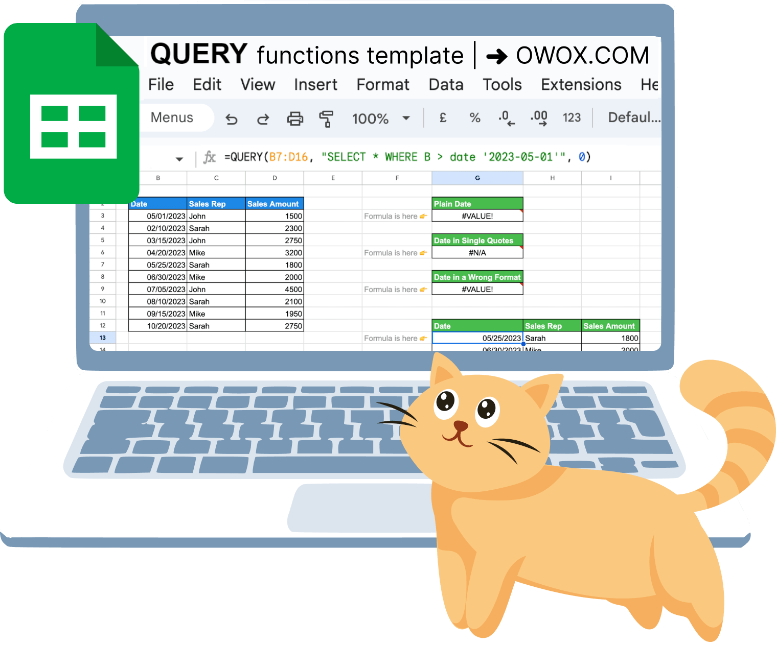
Example #1: Error with Plain Date
You might start by writing the following query:
=QUERY(B2:D12, "SELECT * WHERE B > 05/01/2023", 0)
Here's the formula breakdown:
- QUERY(B2:D12, ...): The QUERY function is used to extract specific data from a range (B2:D12) based on conditions you define.
- Extracts data from the range based on the specified condition.
- "SELECT * WHERE B > 05/01/2023": SELECT * means "select all columns" from B2:D12 and WHERE B > 05/01/2023 sets the condition for date filtering.
- 0: The final argument, 0, tells Google Sheets that there are no headers in the selected range (B2:D12). So, it treats all rows, including the first row, as data instead of headers.

However, this formula triggers a #VALUE! error.
Example #2: Error with Date in Single Quotes
Next, you may try adding single quotes around the date:
=QUERY(B2:D12, "SELECT * WHERE B > ‘05/01/2023’", 0)

In this case, the QUERY function returns a #N/A error or no results because Google Sheets is interpreting '05/01/2023' as a text string, not a date value, resulting in a malfunctioning query.
Example #3: Error with Date in the Wrong Format
Even when using the correct "date" parameter, you may still run into issues if the date format is incorrect:
=QUERY(B3:D12, "SELECT * WHERE B > date '05/01/2023'", 0)

Here, the date is still not recognized because it is not in the required format.
Example #4: Correct Date Filtering Manually
To filter by date successfully, you need to format the date correctly:
=QUERY(B7:D16, "SELECT * WHERE B > date '2023-05-01'", 0)

This formula works because the date is in the required YYYY-MM-DD format, giving the expected result. However, this approach is manual. What happens when you're dealing with large datasets that require more dynamic filtering?
Handling dates correctly in the QUERY function can be tricky, often leading to frustrating results when dates are misinterpreted as text. Understanding the causes behind these issues is the first step.
In the following sections, we will walk you through detailed, step-by-step strategies to ensure your queries work flawlessly with date filters. Let’s dive into the methods that will help you fix these issues and filter your data correctly.
Step-by-Step Guide to Date Filtering Using QUERY
The Query function in Google Sheets is one of the program's most powerful and versatile features. With this tool, you can manipulate data in Google Sheets using a variety of data commands. It can replicate much of the functionality of pivot tables, effectively replacing several other functions.
By using the Query function to filter data by date range, you can display only the values that fall within a specific period or beyond, providing greater control over your dataset.
💡The FILTER function in Google Sheets is an essential tool for narrowing down data based on specific criteria, making it easier to focus on the information that matters most. If you want to simplify your data analysis and improve your workflow, check out our detailed guide on the FILTER function and enhance your ability to work efficiently with complex datasets in your spreadsheets

Step 1: Understanding Date Formats
When using the QUERY function in Google Sheets to filter dates, it is crucial to ensure that dates are formatted consistently for accurate filtering. Google Sheets treats dates as serial numbers, which facilitates proper comparisons.
To ensure dates are recognized correctly, convert them to a standard format like YYYY-MM-DD using the TEXT and DATEVALUE functions. This conversion helps avoid issues where dates might otherwise be interpreted as text, ensuring that the QUERY function processes them accurately.
Step 2: Preparing Your Data for Date Filtering
Before applying the QUERY function, your data must be prepared. Make sure the dates are consistent and that your data doesn't mix date formats or include non-date values in the date column. For example, mixing text with date values can cause errors when filtering.
If you plan to filter your data by a range of dates, ensuring all entries in the date column are correctly formatted is key. You may also want to separate your data into different sections if it contains complex information, such as multiple date columns or varying formats.
Step 3: Formatting Dates with TEXT Function
In some cases, your dates might not be in a consistent format or may need to be formatted explicitly for the QUERY function to work correctly. The TEXT() function can help in this situation, ensuring dates are formatted as YYYY-MM-DD.
Let's use this formula here:
=ARRAYFORMULA(TEXT(B3:B12, "yyyy-mm-dd"))
Let's break down the components of the formula:
- ARRAYFORMULA(...): This allows you to apply a function to a range of cells rather than a single cell. Without it, the TEXT function would only convert the date in one cell.
- TEXT: This function converts a date value into a text string with a specific format.
- B3:B12: This represents the range of cells that contain the original dates. Each value in this range will be converted.
- "yyyy-mm-dd": It specifies the desired format for the dates.

This converts the dates in column B into the required format. This is helpful when you're working with dates stored in different formats across your dataset. While TEXT converts dates into strings for display purposes, it helps to standardize them before applying the QUERY function, ensuring that all dates are comparable.
Step 4: Crafting the QUERY Function
Once your data is prepared and your dates are formatted consistently, you can use the QUERY function. Let’s say you want to filter for all sales made after July 1, 2023.
The QUERY function would look like this:
=QUERY(B2:D12, "SELECT * WHERE B > date '" & TEXT(DATEVALUE("07/01/2023"), "yyyy-mm-dd") & "'", 0)
Here’s how it works:
- B2:D12: refers to your data range, which includes columns for Date, Sales Rep, and Sales Amount.
- SELECT * WHERE B > date '...: selects all rows where the value in column B is greater than July 1, 2023.
- TEXT(DATEVALUE("07/01/2023"), "yyyy-mm-dd"): converts and formats the date properly for comparison.
- 0: indicates that there is no header row in the selected data range.
Using the date keyword ensures that the comparison is made against actual date values rather than text strings.
Step 5: Executing Your QUERY Formula
Once you've crafted the formula, it's time to execute it. Running the following formula:
=QUERY(B2:D12, "SELECT * WHERE B > date '" & TEXT(DATEVALUE("07/01/2023"), "yyyy-mm-dd") & "'", 0)

This result displays all sales made after July 1, 2023. The QUERY function successfully filters out dates before the specified date, returning only the relevant rows.
By following these steps, you can easily filter your data using the QUERY function in Google Sheets, applying date conditions to extract the most relevant information.
💡Combining QUERY with the CONCATENATE function in Google Sheets unlocks powerful ways to merge and analyze data efficiently. Mastering this combination can help you create more dynamic queries and handle complex datasets with ease. Check out our detailed guide on using QUERY with CONCATENATE to take your data analysis to the next level and make more informed decisions in your spreadsheets.

More Useful Date Filtering Techniques in QUERY
The QUERY function in Google Sheets offers powerful date filtering techniques like referencing a date in a cell, filtering between two dates, and using today's date dynamically. These methods provide flexibility and precision in analyzing specific timeframes efficiently.
Referencing a Date in a Cell
Referencing a date stored in a separate cell allows greater flexibility when filtering data using the QUERY function. This approach makes it easy to adjust the filter criteria without editing the formula, which is especially useful for frequently updated reports.
For example, suppose you want to filter your dataset to show sales that occurred after a specific date stored in cell H10. If cell H10 contains the date 06/1/2023, you can use the following formula:
=QUERY(B2:E12, "SELECT * WHERE B > date '" & TEXT(DATEVALUE(H10), "yyyy-mm-dd") & "'", 0)
In this example:
- B2:E12: is the range containing the dataset, including columns for Date, Sales Rep, Region, and Sales Amount.
- H10: is the cell containing the date that will be used as the filter criterion.
- TEXT(DATEVALUE(H10), "yyyy-mm-dd"): converts the date in H10 to the required format for the query, ensuring Google Sheets recognizes it correctly.

This approach makes it easy to modify the filter by changing the value in H10.
Filter Between Two Dates
Filtering between two dates is a common requirement when analyzing data over a specific period. This helps narrow down the dataset to a defined date range, allowing you to focus on relevant entries. This is also known as filter by date range.
Suppose you want to filter the sales that occurred between May 1, 2023, and August 1, 2023. You can use the following QUERY function:
=QUERY(B2:E12, "SELECT * WHERE B >= date '" & TEXT(DATEVALUE("05/01/2023"), "yyyy-mm-dd") & "' AND B <= date '" & TEXT(DATEVALUE("08/01/2023"), "yyyy-mm-dd") & "'", 0)
In this example:
- QUERY: this function is used to filter rows from B2:E12.
- "SELECT * WHERE B >= date '...: this condition filters for rows where the date in column B falls between May 1, 2023, and August 1, 2023.
- TEXT(DATEVALUE("...")): this condition converts the given date into the YYYY-MM-DD format, ensuring proper interpretation.

This filtered dataset includes only the sales that happened between the specified dates, making it easier to analyze trends within that time frame.
Using Today's Date as a Filter
Sometimes, you may need to filter your dataset based on today's date, such as finding all sales that occurred before or after today. This dynamic filtering is useful for reports that need to be updated daily without manual intervention.
To filter the dataset to show all sales after today’s date, you can use the TODAY() function combined with the QUERY function:
=QUERY(B2:E12, "SELECT * WHERE B > date '" & TEXT(DATEVALUE(TODAY()), "yyyy-mm-dd") & "'", 0)
In this example:
- B2:E12: is the data range.
- TEXT(DATEVALUE(TODAY()), "yyyy-mm-dd"): converts today's date into the required YYYY-MM-DD format for the query.
- "WHERE B > date ...": ensures that only the rows with a date after today are returned.

This approach is incredibly useful for tracking upcoming events or filtering for recent activities, allowing your report to stay up to date automatically.
By utilizing these different date filtering techniques in the QUERY function, you can dynamically adjust and refine your dataset, ensuring that only the most relevant information is presented for your analysis. Whether referencing a specific cell, filtering between two dates, or using today’s date, these methods help you maintain efficient and flexible data management in Google Sheets.
Best Practices for Date Filtering in Google Sheets with the QUERY Function
To achieve accurate results when filtering dates, ensure consistent date formatting, use dynamic references where applicable, and validate query results. Proper date handling and correct use of operators are essential for effective filtering in Google Sheets.
Use the DATE Clause
The DATE clause is essential when you need to filter data by dates within the QUERY function. It ensures that the date values are interpreted correctly, preventing errors and enabling accurate comparisons.
Always use the date keyword when specifying a date in the QUERY function, such as date '2023-05-01'. This clearly indicates to Google Sheets that the value is a date and not a text string, which is essential for accurate filtering and obtaining the expected results. Using the TEXT and DATEVALUE functions further helps in formatting dates properly for reliable filtering.
Apply Correct Date Formatting
To ensure the QUERY function processes dates correctly, all dates must be formatted in the standard ISO format (yyyy-mm-dd). This uniformity prevents errors and ensures accurate comparisons, as Google Sheets may misinterpret inconsistent date formats as text or return unexpected results.
Using the TEXT() and DATEVALUE() functions helps convert dates into the correct format, especially for dynamic filtering with functions like TODAY(). Always verify that your date column is properly formatted as dates, which facilitates reliable and accurate data analysis.
Enclose Dates in Single Quotes
When specifying dates in your QUERY string, always enclose them in single quotes (') to indicate that they are date values, not numbers. This distinction is crucial because the QUERY function requires dates to be formatted as strings in the yyyy-mm-dd format. For instance, use "WHERE B > date '" & TEXT(DATEVALUE("05/01/2023"), "yyyy-mm-dd") & "'" in your query.
Failing to use single quotes can lead to errors or incorrect results, as Google Sheets may misinterpret the input as a numerical value. By correctly enclosing dates in single quotes, you ensure that the QUERY function accurately processes the date value, enabling precise and reliable filtering in your data analysis.
Powerful Google Sheets Functions for Advanced Data Analysis
Mastering key functions in Google Sheets can transform the way you handle large datasets, making analysis faster and more accurate. The following functions are essential for streamlining your data workflows and uncovering valuable insights.
- VLOOKUP: Searches for a value in the first column of a table and returns a corresponding value from another column, perfect for quickly finding related information across datasets.
- UNIQUE: Identifies and removes duplicate entries, providing a list of distinct values to ensure cleaner, more focused data analysis.
- PIVOT: Creates pivot tables that summarize large datasets, organizing and calculating data automatically to provide a high-level view of key metrics.
- DATE: A set of functions for managing dates, including DATE for creating valid dates, EDATE for adjusting by months, DATEVALUE for converting text to dates, DATEDIF for calculating date differences, and EPOCHTODATE for converting epoch time to readable dates.
- MATCH: Finds the relative position of a specific value within a range, often used with other functions like INDEX to perform dynamic lookups.
- COUNTA: Counts all non-empty cells in a range, giving you a quick overview of the data size, including text and numeric values.
- AVERAGE: Calculates the mean of a set of numbers, helping you identify central trends and patterns in your data.
These functions empower you to manage large datasets effectively, enabling you to process, analyze, and extract insights with ease.
Instantly Visualize Your Data with OWOX: Reports, Charts & Pivots Extension
Effortlessly turn your raw data into insightful visuals with the OWOX: Reports, Charts & Pivots Extension for Google Sheets. With just a few clicks, you can create dynamic reports, compelling charts, and detailed pivot tables – all within the familiar interface of Google Sheets.
This powerful extension enables you to quickly visualize data trends, understand key metrics, and derive actionable insights. Whether you're a data analyst or a marketer, OWOX: Reports, Charts & Pivots Extension makes it easy to simplify complex data, improve your analytics workflow, and make informed, data-driven decisions.
Frequently asked questions


Finally, a tool that doesn't ask business users to learn a new dashboarding UI. Our marketing team already knows Sheets. OWOX just delivers the right data.
Joinable data marts concept was the thing that sold us. We can now use the semantic layer without building one.
Self-hosted the OSS version on Digital Ocean. Zero vendor lock-in. Contributed a Shopify connector back in week two.