Understanding Star Schema: Guide with Examples

Imagine a business with vast amounts of sales, customers, and product data scattered across multiple systems. Analysts need to extract meaningful insights, but every query feels like navigating a maze of complex relationships. Without an efficient structure of business-ready data, extracting insights becomes time-consuming, delaying decision-making.

This is where the star schema comes in. Designed for speed and simplicity, it streamlines data retrieval, enhances query performance, and supports business intelligence. In this guide, we’ll explore its fundamentals, key components, and how it compares to another popular type of data modeling schema - the snowflake schema.

What is Star Schema in Data Modeling?

A star schema is a data modeling approach designed for organizing information in a structured and efficient way. 

It is commonly used in data warehouses, databases, and data marts to simplify querying and analysis. The design centers around a fact table linked to multiple dimension tables, creating a star-like structure.

It’s also known as Kimball data model, because it was developed by Ralph Kimball in the 1990s. The star schema helps store large datasets efficiently while maintaining historical data. 

By reducing redundant business definitions, it enables faster data aggregation and filtering, making it a preferred choice for business intelligence and reporting.

Example of Star Schema in Data Warehousing

Suppose a retail company wants to track sales performance across various stores, products, and customer segments. It organizes sales transaction data using a star schema for faster queries and efficient reporting.

In this schema, the Sales_Fact table records sales transactions with key details like quantity sold, revenue, and discounts.

It connects to four dimension tables:

• Customer_Dimension (Customer details)
• Product_Dimension (Product information)
• Time_Dimension (Sales date hierarchy)
• Store_Dimension (Store locations)

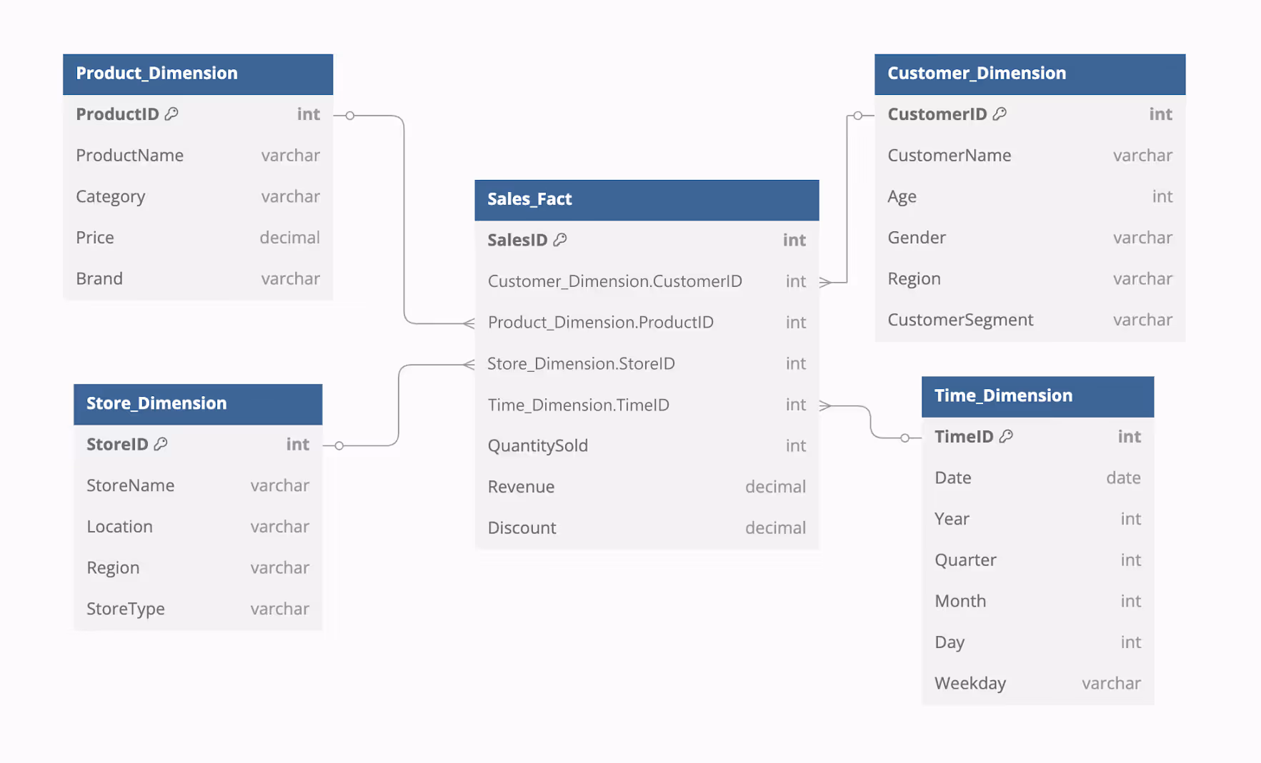
This structure simplifies reporting, allowing quick insights into sales trends, customer behavior, and product performance across different regions and time periods.

Components of a Star Schema 

A star schema consists of key components that structure data for efficient analysis and reporting. These include fact tables, dimension tables, attributes, and attribute hierarchies, each playing a crucial role in data organization.

Fact Table

At the center of a star schema, a fact table stores numerical data reflecting business performance. It contains measurable values (facts) and foreign keys that link to dimension tables, enabling detailed analysis. These tables are periodically updated with aggregated data and support summarization for reporting.

The granularity of a fact table determines the level of detail stored, such as daily or monthly sales figures. Since fact tables typically have a high number of rows but fewer columns, they ensure efficient data storage and retrieval.

Example:

Imagine you're managing a retail business and need to analyze sales performance. The Sales Fact Table records each transaction and includes –  Product ID, Customer ID, Store ID, Date Key, Quantity Sold, and Total Sales Amount – The revenue from the transaction.

Since the fact table stores numerical data, businesses can quickly track monthly revenue trends, best-selling products, or regional sales performance. By joining it with dimension tables, reporting and trend analysis become more efficient and insightful.

Dimension Tables

Dimension tables store descriptive information that provides context to the numerical data in a fact table. They contain attributes that help categorize and filter data, supporting detailed reporting and decision-making.

Each dimension table has a primary key that links to the fact table’s foreign key, enabling data grouping and filtering. Unlike fact tables, dimension tables are not highly normalized to avoid complex joins, ensuring faster query execution. Since dimension attributes evolve over time, these tables help maintain historical data, making them essential for business intelligence and trend analysis.

Example:

In a star schema, a dimension table adds descriptive context to the numerical data in the fact table. 

For example, the Product Dimension Table stores details about each product:

• Product ID – Unique identifier (joins with the Fact Table).
• Product Name – e.g., "Wireless Headphones."
• Category – e.g., "Electronics."
• Brand – e.g., "Sony."
• Price – Standard product price.

By linking to the Sales Fact Table, businesses can analyze sales by category, top-selling brands, and product performance across regions, making reports more insightful.

Attributes

Attributes are descriptive columns in a dimension table that provide detailed information about an entity. They help categorize, filter, and analyze data, making it easier to generate insights for decision-making.

Example:

Each dimension table contains specific attributes:

• In the Product Dimension Table, Product Category and Brand classify products.
• In the Customer Dimension Table, Customer Region and Customer Segment help group customers by location and demographics.

These attributes define and describe business data, making it easier to segment and analyze trends.

Attribute Hierarchies

Attribute hierarchies organize data into different levels, allowing users to drill down into detailed data or roll up to view higher-level summaries. They establish a one-to-many (N:1) relationship between hierarchy levels, helping analysts analyze data from different perspectives.

Example:

• A Time Hierarchy in the Time Dimension Table follows this structure:
  Year → Quarter → Month → Day, allowing analysis at various time scales.
• A Location Hierarchy in the Store Dimension Table follows this structure:
  Region → State → City, enabling geographic trend analysis.

These hierarchies refine data exploration, allowing users to track trends at multiple levels and improve business intelligence.

Key Advantages of Using a Star Schema 

Using a star schema offers several advantages for data warehousing and analytics. Its simple structure enhances query performance, improves data retrieval speed, and makes reporting more efficient for business intelligence and decision-making.

Streamlined Business Reporting and Trend Analysis

Unlike highly normalized schemas, the star schema structures data for rapid access to key performance metrics. 

By centralizing numerical data in a fact table and linking it to descriptive dimension tables, businesses can efficiently perform period-over-period comparisons, track monthly sales growth, analyze regional performance trends, and generate quarterly financial reports with minimal processing delays.

Simplified Join Logic for Faster Query Execution

Reducing query complexity is essential for efficient data retrieval, and a star schema helps achieve this by simplifying join logic. Unlike normalized schemas that require multiple table joins, it directly connects fact tables to dimension tables. 

This structure minimizes processing time, enhances query speed, and makes data analysis more accessible for business intelligence and reporting.

Seamless Integration with OLAP Systems

OLAP systems rely on well-structured data models, and a star schema provides an efficient foundation for building analytical cubes. Its straightforward design allows direct integration with OLAP tools, often eliminating the need for additional cube structuring. 

This compatibility enhances data processing, enabling faster multidimensional analysis and more effective business intelligence reporting.

Optimized Query Performance Through Enhanced Execution Plans

Query optimization plays a vital role in improving data retrieval speed. The star schema enables query processors to apply efficient execution plans, reducing processing time and enhancing performance. 

By streamlining data access, it allows businesses to run complex analytical queries faster, making large-scale reporting and decision-making more effective.

Historical Data Retention for Better Forecasting

The star schema efficiently stores and organizes historical data, making it ideal for long-term trend analysis, forecasting, and performance tracking. Businesses can analyze past performance and identify trends to make data-driven strategic decisions.

Intuitive Data Navigation for Business Users

A key advantage of the star schema is its easy-to-understand structure, which enables technical and non-technical users to explore and analyze data without requiring deep SQL expertise. This simplicity reduces dependency on IT teams and improves self-service analytics.

Scalable Structure for Growing Data Needs

As businesses expand, data volume increases. The star schema is designed to handle large datasets efficiently, ensuring that performance remains optimal even as data complexity grows. This scalability makes it suitable for organizations of all sizes.

Alignment with Spreadsheets & BI Tools

Most reporting & BI tools, such as OWOX Reports, Tableau, Power BI, and Looker Studio, are designed to work efficiently with star schemas. 

Its structure simplifies dashboard creation, allowing businesses to visualize data effectively and extract meaningful insights with minimal processing effort.

Key Differences Between Star and Snowflake Schema 

Star and Snowflake schemas are two common data models in data warehousing, each with distinct structures and advantages. The table below outlines their key differences to help determine the best fit.

‍

Designing, Implementing, and Querying a Star Schema 

This section walks through designing, implementing, and querying a star schema using a real-world use case.

A growing e-commerce business wants to improve its sales analytics and reporting by designing a Star Schema. The goal is to track sales transactions, analyze customer behavior, evaluate product performance, and assess regional sales trends.

The central fact table will store transactional data, while dimension tables will provide descriptive details to enhance analysis. The schema will support business intelligence (BI) reporting, trend analysis, and forecasting.

Designing a Star Schema

A Star Schema is a data modeling technique used in data warehouses to optimize querying and reporting. It consists of a central fact table connected to multiple dimension tables, forming a star-like structure.

For our E-commerce Sales Data Warehouse, we will:

• Identify the central fact table that stores quantitative business metrics.
• Design dimension tables that provide detailed context about products, customers, and orders.
• Establish relationships between fact and dimension tables to enable efficient data retrieval.
• Structure attribute hierarchies to support drill-down analysis.

Let’s explore each step in detail.

Selecting the Central Fact Table for Business Metrics

The company wants to track sales transactions, including revenue, discounts, and order quantities. The fact table will store these numeric business metrics, which can be aggregated for analysis. 

The fact table will be named fact_sales and will store transactional data such as:

• Order ID (Unique identifier for each transaction)
• Date ID (Links to the Date Dimension)
• Customer ID (Links to the Customer Dimension)
• Product ID (Links to the Product Dimension)
• Region ID (Links to the Region Dimension)
• Quantity Sold
• Price Per Unit
• Total Sales Amount
• Discount Applied
• Profit

‍

The fact_sales table forms the core of the schema, capturing business performance data.

1Table fact_sales {
2  OrderID        INT   [primary key]
3  DateID         INT   
4  CustomerID     INT  
5  ProductID      INT   
6  RegionID       INT   
7  QuantitySold   INT
8  PricePerUnit   DECIMAL(10,2)
9  TotalSalesAmount DECIMAL(12,2)
10  DiscountApplied DECIMAL(10,2)
11  Profit         DECIMAL(12,2)
12}

‍

Designing Dimension Tables for Detailed Context

To analyze sales effectively, the business needs dimension tables that provide descriptive context about products, customers, regions, and time.

The following step shows designing the different dimension tables i.e. Product, Customer, Region, and Date.

1. Product Dimension (product_dim)

This table stores details about the products being sold.

1Table product_dim {
2  ProductID      INT  [primary key]
3  ProductName    VARCHAR(255)
4  Category       VARCHAR(100)
5  SubCategory    VARCHAR(100)
6  Brand          VARCHAR(100)
7  Supplier       VARCHAR(255)
8  UnitCost       DECIMAL(10,2)
9}

2. Customer Dimension (customer_dim)

This table captures customer details to analyze buyer behavior.

1Table customer_dim {
2  CustomerID     INT  [primary key]
3  FullName       VARCHAR(255)
4  Email          VARCHAR(255)
5  PhoneNumber    VARCHAR(20)
6  LoyaltyStatus  VARCHAR(50)
7  CustomerSince  DATE
8}

3. Region Dimension (region_dim)

This table stores geographical data to track regional sales trends.

Table region_dim {
  RegionID       INT  [primary key]
  RegionName     VARCHAR(100)
  Country        VARCHAR(100)
}

4. Date Dimension (date_dim)

This table stores time-related attributes for trend analysis.

1Table date_dim {
2  DateID         INT  [primary key]
3  Date           DATE
4  Year           INT
5  Quarter        INT
6  Month          INT
7  DayOfWeek      VARCHAR(20)
8}

These dimension tables enrich the fact_sales table by providing detailed business context.

‍

Linking Fact and Dimension Tables for Data Integration

To enable seamless data retrieval, the fact_sales table must establish foreign key relationships with the dimension tables.

Fact-dimension relationships will be established in the following manner-

• fact_sales.CustomerID → customer_dim.CustomerID
• fact_sales.ProductID → product_dim.ProductID
• fact_sales.RegionID → region_dim.RegionID
• fact_sales.DateID → date_dim.DateID

‍

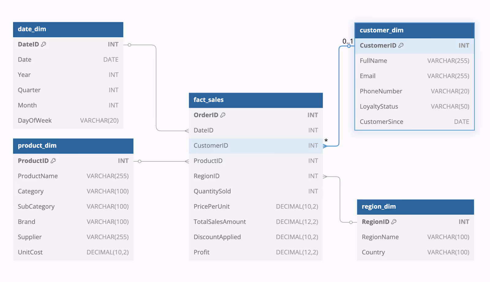
This ensures normalized storage and enables efficient querying by linking transactional data with detailed attributes.

‍

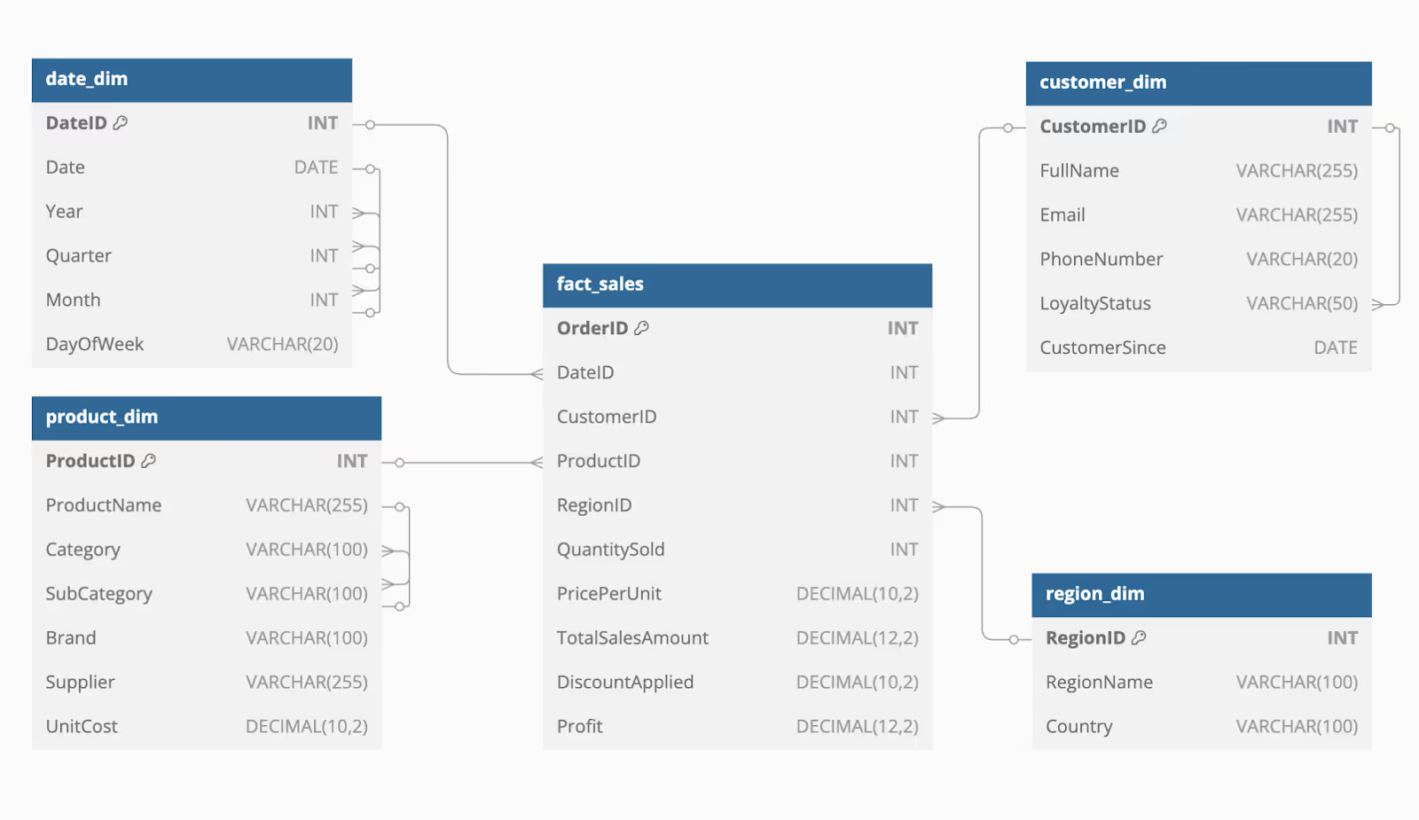
Structuring Attribute Hierarchies for Better Analysis

Suppose the business wants to support multi-level analysis, such as:

• Viewing sales trends by year, quarter, and month.
• Analyzing customer spending by loyalty tiers.
• Grouping products by category and subcategory.

The following steps will ensure the business can create a hierarchical design.

1. Date Hierarchy:

Year → Quarter → Month → Day

Ref: date_dim.Year > date_dim.Quarter
Ref: date_dim.Quarter > date_dim.Month
Ref: date_dim.Month > date_dim.Date

‍

2. Customer Hierarchy:

Loyalty Status → Customer Name

Ref: customer_dim.LoyaltyStatus > customer_dim.CustomerID

‍

3. Product Hierarchy:

Category → Subcategory → Product Name

Ref: product_dim.Category > product_dim.SubCategory
Ref: product_dim.SubCategory > product_dim.ProductName

‍

These hierarchies allow drill-down reports and help uncover business insights efficiently.

‍

Implementing a Star Schema

After designing the Star Schema, the next step is its implementation in a database. This involves:

• Creating fact and dimension tables based on the schema.
• Populating data into these tables to facilitate reporting.
• Optimizing performance using indexing and partitioning.

Creating Fact and Dimension Tables

A Star Schema consists of a central fact table and multiple dimension tables. The fact table stores business metrics, while the dimension tables provide descriptive attributes for analysis.

To implement the schema:

1. Create the fact table (fact_sales): This table contains transactional data, including OrderID, DateID, CustomerID, ProductID, RegionID, Quantity Sold, and Sales Amount.
2. Create dimension tables (date_dim, customer_dim, product_dim, region_dim): Each dimension table provides detailed context for the fact table.
3. Establish relationships between the fact and dimension tables using foreign keys.

Syntax:

1CREATE TABLE Sales (
2    SaleID INT PRIMARY KEY,
3    CustomerID INT,
4    ProductID INT,
5    DateID INT,
6    LocationID INT,
7    Quantity INT,
8    Price DECIMAL(10,2),
9    TotalAmount DECIMAL(10,2)
10);

Key Considerations:

• The fact table should have a highly normalized structure to avoid data duplication.
• Dimension tables should include hierarchies where applicable (e.g., Year → Quarter → Month in date_dim).
• Constraints (such as Primary Keys and Foreign Keys) should be enforced to maintain data integrity.

Once these tables are set up, the next step is loading data into them.

‍

Populating Data into the Tables

Populating data is critical for enabling meaningful analysis. The data load process involves:

1. Extracting Data: Pull data from transactional databases, APIs, or flat files (CSV, JSON, etc.). Ensure the extracted data is clean and structured before loading.
2. Transforming Data: Convert raw data into a structured format that aligns with the schema. Standardize data types (e.g., dates in YYYY-MM-DD format, numeric fields formatted correctly). Resolve missing values and correct any inconsistencies.
3. Loading Data into Tables: Insert transactional data into the fact table (fact_sales). Populate descriptive attributes into dimension tables (e.g., customer_dim, product_dim). Ensure foreign key relationships are maintained.

Syntax:

1INSERT INTO Sales (SaleID, CustomerID, ProductID, DateID, LocationID, Quantity, Price, TotalAmount)
2VALUES (1, 101, 5001, 20240201, 301, 2, 499, 998);

After successfully populating data, the next step is optimizing query performance using indexing and partitioning.

‍

Indexing and Partitioning for Performance Optimization

As the dataset grows, querying the fact table can become slower. To ensure efficient data retrieval, indexing and partitioning techniques should be applied.

1. Indexing for Faster Queries

Indexes improve query performance by allowing the database to locate rows quickly without scanning the entire table.

• Primary Indexes: Applied to primary keys (e.g., OrderID in fact_sales).
• Foreign Key Indexes: Indexing foreign keys (e.g., CustomerID, ProductID) speeds up JOIN operations.
• Composite Indexes: Combining multiple columns in an index improves search performance when filtering by multiple conditions (e.g., DateID, RegionID together).

2. Partitioning for Large Datasets

Partitioning splits large tables into smaller, more manageable pieces, improving query efficiency.

• Range Partitioning: Used for time-series data (e.g., partitioning fact_sales by Year or Month).
• List Partitioning: Useful when dividing data by categorical values (e.g., region-based partitioning).
• Hash Partitioning: Distributes data evenly, reducing query bottlenecks.

Syntax:

1CREATE INDEX idx_sales_date ON Sales(DateID);

‍

Querying a Star Schema in an E-commerce Data Warehouse

One of the key advantages of a Star Schema is its simplicity and efficiency in querying data. By leveraging the structured relationships between the fact table and dimension tables, businesses can easily retrieve, aggregate, and analyze sales data.

Following are some common query operations in an e-commerce Star Schema.

Simple Joins: Retrieving Sales Data with Product and Time Information

To analyze e-commerce sales transactions, we often need to join the fact table (fact_sales) with dimension tables (product_dim, date_dim) to retrieve detailed insights.

Example: Querying Sales by Product and Date

1SELECT f.OrderID, p.ProductName, d.FullDate, f.QuantitySold, f.TotalSalesAmount
2FROM fact_sales f
3JOIN product_dim p ON f.ProductID = p.ProductID
4JOIN date_dim d ON f.DateID = d.DateID;

 What This Query Does:

• Retrieves order details (OrderID, QuantitySold, TotalSalesAmount).
• Joins with product_dim to get the product name.
• Joins with date_dim to fetch the transaction date.
• Provides a comprehensive view of sales transactions.

‍

Aggregations and Roll-ups: Summarizing Sales 

Data Aggregations allow businesses to calculate key metrics such as total revenue, average order value, and total units sold. Roll-ups help summarize sales trends at different levels (e.g., daily → monthly → yearly).

Example: Monthly Sales Aggregation

1SELECT d.Year, d.Month, SUM(f.TotalSalesAmount) AS TotalRevenue
2FROM fact_sales f
3JOIN date_dim d ON f.DateID = d.DateID
4GROUP BY d.Year, d.Month
5ORDER BY d.Year, d.Month;

What This Query Does:

• Aggregates total sales revenue (SUM(f.TotalSalesAmount)) for each month and year.
• Groups data using date attributes from the date_dim table.
• Helps analyze monthly revenue trends for better forecasting.

‍

Drill-down and Drill-up Operations: Navigating Sales Hierarchies

Drill-down and drill-up operations allow analysts to switch between high-level summaries and detailed breakdowns. This helps businesses track performance trends at different granularities.

Example: Quarterly Sales Analysis

1SELECT d.Year, d.Quarter, SUM(f.TotalSalesAmount) AS TotalRevenue
2FROM fact_sales f
3JOIN date_dim d ON f.DateID = d.DateID
4GROUP BY d.Year, d.Quarter
5ORDER BY d.Year, d.Quarter;

What This Query Does:

• Groups sales data by year and quarter to show quarterly revenue trends.
• Helps identify seasonal sales patterns (e.g., holiday shopping spikes).
• Supports strategic decision-making for inventory and marketing campaigns.

‍

Filtering and Slicing Data: Focusing on Specific Product Categories and High-Value Sales

Filtering and slicing allow businesses to analyze specific subsets of data, such as top-selling categories, high-value orders, or region-specific sales trends.

Example: Filtering High-Value Sales for a Specific Product Category

1SELECT p.ProductName, f.QuantitySold, f.TotalSalesAmount
2FROM fact_sales f
3JOIN product_dim p ON f.ProductID = p.ProductID
4WHERE p.Category = 'Electronics' AND f.TotalSalesAmount > 500;

What This Query Does:

• Filters sales transactions for Electronic products.
• Selects orders where the total sales amount exceeds $500.
• Helps identify high-value transactions for targeted promotions.

Tools for Implementing Star Schema in Data Warehousing 

Implementing a star schema requires specialized tools for data integration, storage, and analysis. These tools help streamline data processing, optimize performance, and ensure efficient querying for business intelligence and reporting.

ETL and Data Integration Tools

ETL and data integration tools play a crucial role in structuring data for a star schema. Solutions like Informatica PowerCenter, SSIS, and Talend extract data from source systems, transform it into the required format and load it into the data warehouse. These tools ensure smooth data flow, maintain consistency, and optimize performance for efficient querying and reporting.

Business Intelligence and Analytics Tools

Analyzing star schema data becomes easier with tools that support visualization and reporting. Tableau, Power BI, QlikView, and OWOX BI enable users to connect to data warehouses, run queries, and create interactive dashboards. These platforms help transform raw data into meaningful insights, making business analysis more accessible and efficient for decision-making.

Data Warehouse Platforms

Storing and querying star schema data efficiently requires robust data warehouse platforms. Snowflake, Amazon Redshift, and Microsoft Azure Synapse Analytics provide scalable and high-performance environments for managing large datasets. These platforms optimize storage, improve query execution, and support seamless integration with analytics tools, making them ideal for business intelligence and data-driven decision-making.

Best Practices for Designing Star Schemas 

Designing an effective star schema requires following best practices to ensure optimal performance and scalability. Proper structuring improves query speed, simplifies data management, and enhances reporting for better business intelligence and analytics.

Selecting the Appropriate Level of Granularity

Granularity defines the level of detail stored in the fact table, impacting data analysis and query performance. Selecting the right granularity ensures that data is neither too detailed nor overly aggregated.

It should align with business needs, query patterns, and storage constraints. A lower granularity provides more detailed insights, while a higher one simplifies analysis but may lose specific details.

Structuring Dimension Tables with Normalization 

Organizing dimension tables with normalization helps reduce redundancy and maintain data integrity. It involves breaking down tables into smaller ones based on relationships, ensuring a structured and efficient data model.

Normalized dimension tables prevent duplication, simplify maintenance, and support hierarchies for better analysis. They also enable conformed dimensions, ensuring consistency across multiple fact tables for accurate reporting.

Simplifying Fact Tables Through Denormalization 

Denormalizing fact tables improves query performance by reducing the need for complex joins. This process involves merging data from multiple tables, increasing redundancy while optimizing retrieval speed.

A denormalized fact table simplifies queries, enhances processing efficiency, and supports pre-calculated measures, which store derived values to reduce computation time. This approach is ideal for faster analytics and reporting. 

Utilizing Surrogate Keys for Better Data Management 

Surrogate keys are unique, sequential identifiers assigned to each row in a table, replacing natural keys for better data management. They ensure stability and consistency by remaining unchanged even if source data updates.

Using surrogate keys in fact and dimension tables prevents key conflicts, improves indexing efficiency, and enhances query performance, making data retrieval faster and more reliable.

Handling Slowly Changing Dimensions Effectively 

Slowly changing dimensions (SCDs) are attributes in dimension tables that evolve over time, such as a customer’s address or membership status. Managing these changes is crucial to maintaining data accuracy and historical consistency.

Common strategies include overwriting old values, adding new rows, creating extra columns, or using separate tables, depending on business requirements and the frequency of updates. 

Ensuring Accuracy Through Validation and Testing  

Ensuring the star schema is accurate and consistent requires thorough testing and validation. This process verifies data quality, integrity, completeness, and performance to meet business requirements effectively.

Techniques like data profiling, cleansing, auditing, and reconciliation help identify errors, while testing methods such as data sampling and query validation ensure reliable reporting and secure data management.

Simplify Star Schema Implementation with OWOX BI

Designing a star schema improves query performance, enhances reporting accuracy, and simplifies data navigation, but managing complex data models manually can be time-consuming. 

OWOX BI automates this process, ensuring seamless data integration and eliminating inconsistencies across fact and dimension tables.

By leveraging OWOX BI, analysts can focus on insights rather than troubleshooting data structures. 

Whether you're building a star schema, snowflake schema, or hybrid data model, OWOX BI provides the flexibility and automation needed to scale analytics while maintaining reporting accuracy. 

Try OWOX BI today to optimize your data modeling and business intelligence workflows.