Comprehensive Guide to AVERAGE Functions in Google Sheets

Numbers tell a story, but without the right context, they may lead to confusion rather than clarity. In the world of data analysis, understanding how to process figures accurately is essential for informed decision-making. Google Sheets offers a powerful suite of functions, including AVERAGE functions, designed to simplify this process, making it easier to get valuable insights from your data.

The AVERAGE function is one of the most frequently used tools in Google Sheets, allowing users to calculate the mean of a range with ease. Beyond simple calculations, advanced features such as AVERAGEIF and AVERAGEIFS enable users to apply conditional logic, filtering data based on specific criteria to deliver precise results.

This in-depth guide aims to highlight the nuances of these powerful functions, equipping users with the knowledge to enhance their data analysis capabilities.

Calculating averages is an essential aspect of data analysis, and Google Sheets offers a variety of built-in functions to simplify this task. The AVERAGE function is one of the most straightforward and effective tools for determining the central tendency of a dataset. It calculates the arithmetic mean by summing the values in a specified range and dividing by the number of cells containing numeric data.

This function is ideal for practical applications, such as tracking student grades, calculating average sales, or managing monthly expenses. However, it's important to note that while the AVERAGE function automatically excludes blank cells from the calculation, it does include cells with a value of zero, which can influence the result depending on the context.

The AVERAGE function in Google Sheets efficiently calculates the mean of a specified range of cells. It simplifies the process of finding the central value in your data, reduces manual errors, and automatically adjusts the average as the data changes.

The syntax for the AVERAGE function in Google Sheets is:

Let's break down what these parameters mean:

• value1: The first number or range from which to calculate the average.
• [value2, ...]: Additional numbers or ranges you can include in the average calculation.

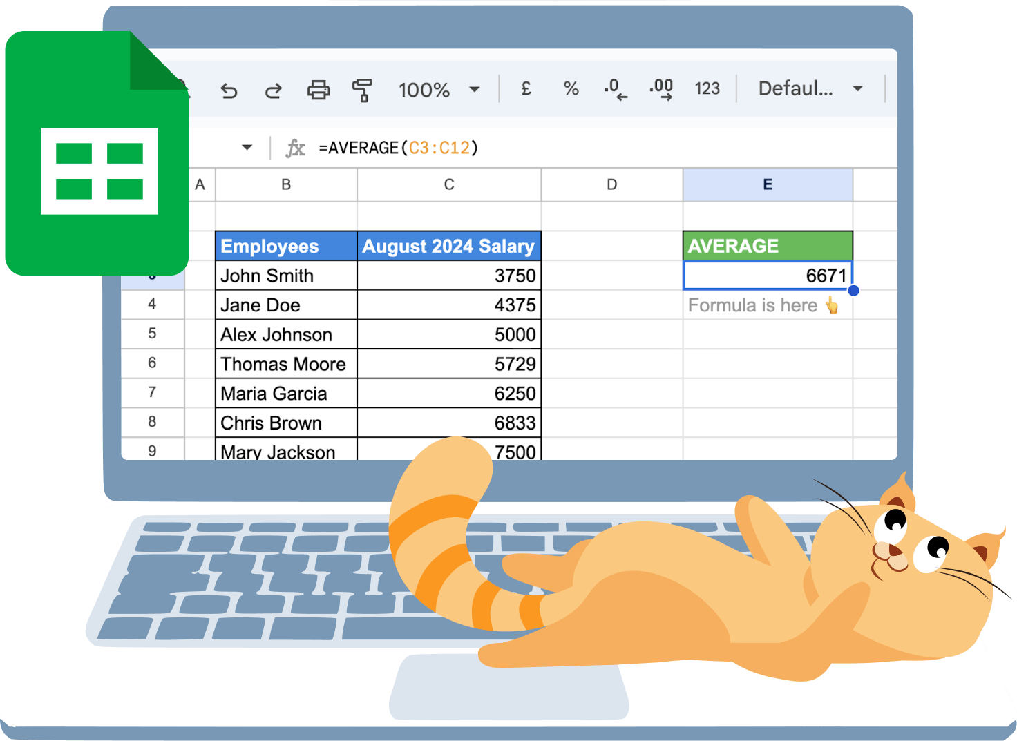
Let's say we have a list of the salaries for 10 employees for August 2024 and would like to find out their average salary in column C.

To calculate this, use the following formula:

Here's the breakdown:

• C3:C12: this is a range in column C, which contains the salary data for the 10 employees.

Adjust the range as needed to match the exact cells where your data is stored.

The AVERAGEA function in Google Sheets calculates the average of a range, including both numbers and text. Unlike the AVERAGE function, AVERAGEA treats text values as 0 and counts them in the average, making it useful when working with mixed data types.

This function helps you understand the overall average, even when non-numeric data is present in your dataset.

The syntax for the AVERAGEA function in Google Sheets is:

Let's break down what these parameters mean:

• value1: The first number, text, or range considered when calculating the average with the AVERAGEA function.
• [value2, ...]: Extra numbers, text, or ranges that can also be included in the AVERAGEA calculation.

Let's say we have the same list of the salaries for 10 employees for August 2024 and would like to find out the average salary in column C.

Since the AVERAGEA function works with numeric values just like the AVERAGE function, we can replace one of the values with a text string to observe how it affects the calculation.

To clarify the difference, let's first explore how the AVERAGE function works with text values.

Here's the formula to use:

Now let's see how the AVERAGEA function works with the same dataset:

As we can see, if one of the values is converted to text, the AVERAGE function ignores it while the AVERAGEA function treats the text as 0, resulting in a different final average.

This difference in how the two functions handle text results in significantly different outcomes. It’s important to choose the function that best suits your data and the analysis you want to perform.

The AVERAGEIF function in Google Sheets is designed to calculate the average of a range of values that meet a specific condition. By including only the numbers that satisfy the given criteria.

It is particularly useful when you need to find the average of data points that match certain conditions, such as values above a set threshold or those linked to a particular category.

The AVERAGEIF function in Google Sheets has the following syntax:

Let us break down its arguments:

• criteria_range: Refers to the group of categories that includes the specific criterion to be averaged.
• criterion: The condition that will be evaluated against the criteria_range, which can be a number, text, date, or expression.
• average_range: An optional argument that holds the values to be averaged.

💡The AVERAGEIF function in Google Sheets is a powerful tool for calculating conditional averages based on specified criteria. However, understanding the foundational logic of the IF function is crucial, as it can help you create more complex conditional formulas beyond just averaging. You can efficiently manage and analyze data in Google Sheets by mastering both functions.

For example, let's add the departments where the employees work to the existing table. By selecting the 'Marketing' department as the criterion, we can use the AVERAGEIF function to calculate the average salary of employees in that department for August 2024.

To calculate the average salary of employees in the 'Marketing' department, use the following formula in Google Sheets:

Here's the breakdown:

• C3:C12: The range of cells to evaluate against the criterion.
• "Marketing": The criteria to apply.
• D3:D12: The range of cells to average.

The AVERAGEIFS function in Google Sheets is a powerful tool for calculating the average of a range based on multiple conditions. Unlike AVERAGEIF, which allows only a single criterion, AVERAGEIFS lets you specify multiple criteria across different ranges. This makes it ideal for more complex analyses where you need to average data that meets several specific conditions.

The syntax for the AVERAGEIFS function is:

The formula requires three parameters to work. These are:

• avg_range: This parameter specifies the cell range that the AVERAGEIFS formula in Google Sheets will average. Unlike the AVERAGEIF formula, where this parameter appears later, in AVERAGEIFS, it comes first.
• crit_range1: This is the cell range that the formula will evaluate based on the condition defined by the criterion1 parameter.
• criterion1: This parameter sets the condition that the cells in crit_range1 must meet to be included in the average. You can use six different comparison operators that we will describe in detail in one of the examples below.
• [crit_range2, criterion2, ...] (optional): Additional ranges and criteria.

💡While the AVERAGEIF function expertly handles conditional averages, the IFS function in Google Sheets provides a streamlined approach for multiple conditions. Dive into our comprehensive guide on the IFS function to expand your capabilities in handling complex data scenarios efficiently.

For example, let's add the KPI performance percentage to the existing table of employees and salaries. We can then calculate the average salary of employees in the 'Marketing' department whose KPI performance is above 70%.

Use the following formula in Google Sheets to make this calculation:

Here's the breakdown:

• C3:C12: The range of cells to average.
• B3:B12: The range of cells to evaluate against the criterion.
• "Marketing": The criteria to apply.
• D3:D12: The range of cells to evaluate against the criterion.
• ">70": The criteria to apply.

Practical examples of using the AVERAGE functions highlight their utility in data analysis. Whether you're calculating the average sales, determining grades, or analyzing performance metrics, these functions simplify the process. By applying AVERAGE for purely numeric data and AVERAGEA for mixed data types, you can efficiently gain insights and make informed decisions.

The AVERAGE function in Google Sheets enables you to calculate the average of values scattered across non-adjacent cells. Instead of averaging a continuous range, you can choose specific cells or ranges by separating them with commas. This approach allows you to accurately compute the mean of selected data points, even when they're spread out across your spreadsheet.

For example, we need to calculate the KPI performance of the sales and marketing departments using the AVERAGE formula.

The formula will look like this:

This flexibility is especially valuable when your data isn't confined to a single block, allowing you to perform accurate calculations without needing to reorganize your spreadsheet. It enables you to efficiently work with scattered data while maintaining the integrity of your original layout.

Combining values and cell references with the AVERAGE function in Google Sheets allows you to calculate the mean of both specific numbers and data within cells.

You can manually input numbers along with cell references in the formula, giving you the flexibility to include both fixed values and dynamic data from your spreadsheet. This approach is useful when you want to average a mix of specific values and cell-stored data in a single calculation.

Suppose we have an additional salary for an employee that hasn't been added to the sheet. We can calculate the average salary of all employees using the following formula:

Such functionality demonstrates the flexibility of the AVERAGE function.

Calculating the average of percentages in Google Sheets is straightforward with the AVERAGE function. This is particularly useful when you need to determine the overall performance across multiple categories. By selecting the range of percentage values, you can quickly find the mean percentage, offering a clear overview of overall performance or trends.

For example, let's add the percentage symbol to the KPI performance values and then attempt to calculate the average.

The formula will look like this:

Calculating average percentages provides a quick and clear insight into overall performance, allowing you to easily assess trends and make data-driven decisions without needing to interpret all percentage values separately.

You can use the AVERAGE function in Google Sheets to calculate the average across multiple columns. By selecting ranges from different columns, the AVERAGE function will compute the mean value for each selected range.

This is particularly useful for analyzing data like monthly sales across different regions or comparing scores across various subjects, helping you gain insights from multiple datasets at once.

To apply this method, we'll add the salaries for July and June to the existing table and calculate the average salary for the summer.

The formula will look like this:

Using the AVERAGE function for multiple columns simplifies data analysis by allowing you to compare and summarize data across various categories at once.

You can use the AVERAGE function across multiple sheets in Google Sheets to calculate the average of data spread over different tabs. This is particularly useful when consolidating data from various sources or time periods.

By referencing specific cells or ranges from different sheets in the AVERAGE formula, you can efficiently combine and analyze data across your entire workbook, providing a more comprehensive view of your dataset.

For example, we have salary figures of John Smith in two different sheets, named 'July 2024 Salary' and 'August 2024 Salary'.

To calculate the average salary for July-August, let's use this formula:

This approach seamlessly merges data from various tabs, simplifying the process of finding an aggregate average when datasets are spread across multiple sheets.

When working with data that includes blank cells, it's essential to understand how the AVERAGE and AVERAGEA functions treat these gaps. Both functions automatically ignore blank cells in your dataset, ensuring that they don't skew the calculated average.

This feature is really useful when dealing with incomplete data, as it allows for accurate analysis without needing to manually adjust for missing values.

For example, let's consider the KPI performance data and calculate the average using both the AVERAGE and AVERAGEA functions. In this case, both functions will produce the same result when there are only blank cells, and no non-numerical data is involved.

Here's how the formula would look using the AVERAGE function:

Here's the formula using the AVERAGEA function:

As you can see, when only blank cells and numerical data are present, AVERAGE and AVERAGEA deliver identical outcomes. This consistency makes it easier to work with datasets where blanks might otherwise complicate your calculations. However, if your data included text values, AVERAGEA would treat them differently by giving them a value of 0, which could impact the result.

Now, let's look at the outcome for the AVERAGEA function when working with Boolean data represented by checkboxes. In this case, we have a list of employees, with checkboxes indicating whether they work from the office.

Google Sheets treats checkboxes as Boolean values, where a checked box represents TRUE, and an unchecked box represents FALSE. Now, we will calculate the average using the AVERAGEA function.

The formula would look like this:

Here, the AVERAGEA function treats a checked box (TRUE) as 1 and an unchecked box (FALSE) as 0. In this example, the AVERAGEA function returns 0.6, meaning that 60% of the employees work from the office.

Using AVERAGEA with Boolean values provides a quick way to quantify the proportion of TRUE values in your data, giving you an easy-to-understand percentage that can help in decision-making and performance tracking.

The "Explore" feature in Google Sheets allows you to quickly average data without manually entering formulas. By simply highlighting your data range and clicking the "Explore" button at the bottom right, Google Sheets automatically suggests calculations, including averages.

This feature is especially useful for quick analyses, saving you time and effort by providing instant insights without needing to write out the AVERAGE function yourself.

For this example, we will use the same employee salary data from the last example, but instead of using a formula to average the test scores, we will use the "Explore" feature to average.

To average with the "Explore" feature in Google Sheets, follow these steps:

• Select the cells / range of cells to be averaged.
• Click the menu on the bottom right where the calculation is shown, and click "Avg:" which stands for "Average".
• Look at the bottom right of the screen, and the automatically calculated average of the selected cells will be displayed.

The "Explore" feature provides instant averages, saving time and simplifying data analysis, especially for large datasets.

The AVERAGEIF and AVERAGEIFS functions in Google Sheets are powerful tools for applying conditional logic to your data analysis. AVERAGEIF allows you to calculate the average of a range based on a single condition, such as finding the average sales only for a specific product.

AVERAGEIFS expands on this by letting you use multiple conditions, enabling more complex analysis, like calculating the average revenue for a product sold in a particular region during a specific time period. These functions help you derive more targeted insights from your data.

The AVERAGEIF function in Google Sheets allows you to use text as a criterion for calculating averages. For example, you can find the average KPI performance percentage for employees from the Business Development department.

By entering the desired text as the criterion, AVERAGEIF will only include cells that meet this condition in the calculation, making it a valuable tool for analyzing data based on labels, names, or categories.

An example formula would look like:

Using text as a criterion in AVERAGEIF allows you to easily analyze specific categories or labels within your data, providing targeted insights without the need for additional filtering or sorting.

The AVERAGEIF function in Google Sheets can also be used with dates as a criterion, allowing you to calculate averages based on specific time frames. For instance, you can find the average sales for a particular month or after a certain date by setting the date as the condition.

For example, we can calculate the average salary paid on 24/08/2024.

The formula would look like this:

This makes it easy to analyze trends over time or compare performance during specific periods, providing more precise insights from your data.

In addition to numbers and text, the criterion in the AVERAGEIF function can also use comparison operators. Let's first take a look at the comparison operators available in Google Sheets.

There are six comparison operators in Google Sheets:

• Equal to ( = ): Checks if the value on the right matches the value on the left.
• Not Equal to ( <> ): Determines if the value on the right does not match the value on the left.
• Less than ( < ): Checks if the value on the right is smaller than the value on the left.
• Greater than ( > ): Determines if the value on the right is larger than the value on the left.
• Less than or Equal to ( <= ): Checks if the value on the right is either smaller than or equal to the value on the left.
• Greater than or Equal to ( >= ): Compares if the value on the right is either larger than or equal to the value on the left.

Let’s take the previous data. In this example, our objective will be to find the average salary of those who earn less than 6,500.

An example formula would look like:

Using comparison operators in the AVERAGEIF function allows for more precise data analysis, enabling you to tailor calculations to specific conditions and uncover insights that are relevant to your particular needs.

Sometimes, zeros can distort the average you're trying to calculate. AVERAGEIF makes it possible to exclude zeros by setting the criterion such that only non-zero cells are considered.

This is particularly useful when zero values would otherwise skew your results, such as when averaging sales figures or test scores, where zero may indicate missing or irrelevant data.

To ignore zero values, the criteria supplied is "<>0", which means "not equal to zero". For example, let's say that we have a few 0s in the salary column.

Then the formula will look like this:

Using AVERAGEIF to skip zeros ensures a more accurate reflection of your data by excluding irrelevant or missing values, helping you avoid skewed results and gain clearer insights.

In Google Sheets, three main wildcards – the question mark (?), asterisk (*), and tilde (~) – function uniquely with specific formulas, including the AVERAGEIF function.

They are used for filtering when you need to return specific results:

• Question mark (?): Represents a single character
• Asterisk (*): Represents any number of characters.
• Tilde (~): Indicates that a character should be interpreted literally, rather than as a wildcard.

Suppose you want to calculate the average salary of employees starting with a specific name, such as "John."

The formula will look like this:

As a result of this formula, you will get the average salary of only employees whose names start with "John". You can use the question mark wildcard similarly that will replace any single character.

The AVERAGEIFS function in Google Sheets allows you to calculate the average of a range based on multiple conditions, providing a more refined analysis. By specifying multiple criteria, such as date ranges, categories, or thresholds, you can target specific subsets of your data.

This function is particularly useful for complex datasets where you need to analyze averages under several conditions simultaneously, such as finding the average sales for a product during a particular season in a specific region.

In this example, we are going to have multiple conditions. Consider the data from the previous example. Here, we not only want to find out the average salary of employees, but we also want to find out the average salary of employees in the 'Marketing' department, whose KPI performance percentage is less than 80%.

In this case, the formula will look like this:

Using multiple conditions with AVERAGEIFS allows for more targeted and precise analysis, enabling you to focus on specific data subsets and gain deeper insights into complex datasets.

In summary, understanding and correctly applying AVERAGEIF and AVERAGEIFS in Google Sheets empowers users to carry out specific and accurate average calculations, which can substantially aid in data analysis.

Using the AVERAGE function with ARRAYFORMULA in Google Sheets allows you to efficiently calculate group-wise means across a dataset. By applying ARRAYFORMULA, you can automatically extend the AVERAGE function to multiple rows, enabling you to find the mean for each group without manually inputting the formula for each one.

This approach simplifies the process of calculating averages for different categories or groups within your data, saving time and ensuring consistency in your analysis.

For example, you have a table that lists the sales figures for different sales representatives in various regions, and you want to calculate the average sales for each region.

The formula will look like this:

Let's explain the formula:

• IF(D3:D12=F3,C3:C12): This part of the formula checks each cell in the range B3:B12 (which contains the regions) to see if it matches "North" (or whatever region is in F3). If it matches, it returns the corresponding sales figure from range C3:C12.
• ARRAYFORMULA: This allows the formula to handle an array (range of cells) instead of just a single cell.
• AVERAGE: This calculates the average of the sales figures returned by the IF function.

This same formula can be applied to other regions by changing the value in F3 to "South" or "East," and it will calculate the proper averages for those regions.

Using AVERAGE with ARRAYFORMULA to find group-wise averages makes the process much easier and faster. It automatically calculates averages for each group, saving you the hassle of doing it manually and ensuring consistent, accurate results, especially when dealing with lots of data.

💡The ARRAYFORMULA function in Google Sheets is a versatile tool for managing large datasets and automating calculations across multiple cells. To improve your data handling, check out our comprehensive guide on using ARRAYFORMULA, helping you create more efficient and dynamic spreadsheets.

When working with averaging functions in Google Sheets, you may run into common issues that can disrupt your calculations. Problems like errors in the formula or unexpected results often arise, especially when dealing with empty cells, zeros, or incorrect criteria.

Troubleshooting these issues involves carefully checking your data and formulas to ensure everything is set up correctly, helping to maintain accurate and reliable results in your spreadsheets.

When using the AVERAGE function in Google Sheets, you might encounter the #DIV/0! error. This happens because averaging numbers involves division, and dividing by zero is undefined. The error typically occurs when the range you’re trying to average contains no numeric values or is completely empty, leading to a zero denominator.

⚠️ Error: The #DIV/0! error occurs because there are no numeric values in the range, leading the AVERAGE function to attempt dividing by zero.

✅ Solution: Ensure the range contains relevant data, or use this formula:

This method will help you avoid the error message by displaying a custom message if the range is empty.

When working with averages in Google Sheets, a #DIV/0! error can occur if the range you're averaging contains no numeric values. This issue often arises when numbers are mistakenly formatted as text.

⚠️ Error: The #DIV/0! error occurs because the cells you're trying to average are recognized as text instead of numbers.

✅ Solution: To fix the error, simply convert the text-formatted numbers back into numeric values. Select the range, go to Format > Number > Automatic, and Google Sheets will reformat your data to the correct number format.

When using the AVERAGE function, encountering an #N/A error within your data range can cause the function to return the same error in the result as well. This issue arises when some cells in your range contain #N/A errors.

⚠️ Error: The #N/A error occurs because one or more cells in your range have an error, causing the AVERAGE function to fail.

✅ Solution: To bypass this issue, you can use the AVERAGEIF function to ignore the #N/A errors and calculate the average only for valid numerical data.

Here’s how you can do it:

This formula tells Google Sheets to average the values in the range C3:C12, excluding any cells with the #N/A error.

If you want to ignore all types of errors, like '#N/A' or '#DIV/0!', you can adjust the AVERAGEIF criteria:

This version averages only the cells with numbers greater than 0, effectively ignoring any cells with errors or non-numeric values.

To achieve accurate and reliable data averaging in Google Sheets, it's important to follow a few key best practices. Start by integrating relevant functions to handle specific scenarios or streamline calculations.

• Integrate relevant functions to handle specific scenarios or simplify your calculations.
• Ensure data validation is in place to maintain data integrity and prevent errors caused by incorrect inputs.
• Regularly review and update your datasets to catch anomalies, remove outdated data, and keep your averages current.

By adopting these practices, you can maintain precision and effectiveness in your data analysis, ensuring that your results are both accurate and insightful.

Enhance your data analysis by combining the AVERAGE function with other Google Sheets functions. By combining AVERAGE with functions like IF, ARRAYFORMULA, FILTER, and QUERY, you can create more nuanced and powerful calculations that address specific needs in your datasets.

• IF: Average only specific data points based on criteria (e.g., positive numbers).
• ARRAYFORMULA: Apply AVERAGE across multiple rows/columns simultaneously, ideal for large datasets.
• FILTER: Dynamically filter data before averaging, ensuring only relevant data is included.
• QUERY: Use SQL-like queries to pull and average specific data segments, perfect for detailed reports.

By leveraging these integrations, you can enhance the functionality of the AVERAGE function, making your data analysis more efficient, accurate, and adaptable to various scenarios.

Data validation in Google Sheets is critically important for ensuring accurate averages. By controlling the type of data entered, you prevent errors that could skew your calculations.

For example, setting rules to allow only numeric values ensures that non-numeric entries don’t distort your averages. Validation also helps manage blank cells and outliers, maintaining the integrity of your data. Regularly updating these rules keeps your dataset accurate as it evolves.

The =DATAVALIDATION(criteria_range, criterion) function is key to keeping your datasets reliable and ensuring that only the right data is calculated, making your analyses both accurate and dependable.

Regular reviews are essential for maintaining accurate averages and current data. Set a schedule to examine datasets for anomalies or changes, update averages as new data comes in, and remove outdated or irrelevant data points.

Automate parts of this process with scripts or add-ons to save time.

For best practices, review data weekly or monthly, update formulas after significant changes, and clean datasets quarterly. Keeping your data fresh and accurate ensures your averages always reflect the latest trends, making your analysis reliable and relevant.

Google Sheets provides a variety of powerful formulas that can simplify and improve the way you analyze data.

• VLOOKUP: Searches for a value in the first column of a range and returns a value in the same row from a specified column.
• UNIQUE Function: Extracts unique values from a specified range or array, eliminating duplicates.
• Pivot Tables: Summarizes large data sets and allows dynamic reorganization and analysis of data through a tabular format.
• MATCH Function: Returns the position of a specified item in a range.
• COUNT and COUNTA: COUNT calculates the number of cells with numerical data, while COUNTA counts all non-empty cells.
• INDEX and MATCH: Combines INDEX and MATCH functions for advanced lookups, replacing more complex VLOOKUP scenarios.
• COUNTIF and COUNTIFS: COUNTIF performs conditional counts based on a single criterion, and COUNTIFS extends this to multiple criteria.

Data analysis in Google Sheets can be transformed from a mundane task into a streamlined and efficient process by leveraging robust tools and techniques. Begin by harnessing the AVERAGE function to compute mean values within your datasets swiftly.

Enhance your data analysis efficiency with the OWOX: Reports, Charts & Pivots Extension by seamlessly integrating powerful analytics directly within your Google Sheets environment. This extension allows you to optimize the process of querying and analyzing large datasets in BigQuery.

With OWOX Reports, you can automate the extraction, transformation, and loading (ETL) of data, reducing manual effort and ensuring that your reports are always up-to-date. This not only saves time but also enhances accuracy, enabling you to focus on gaining insights and making data-driven decisions.