How to Use the REPLACE Function in Google Sheets for Seamless Text Updates
Manually updating text in large datasets can be time-consuming, but Google Sheets offers a simple solution—the REPLACE function. This powerful tool allows you to modify specific portions of text within a cell based on position and length, making it ideal for correcting data entries, standardizing formats, and making bulk text changes efficiently.

Whether you're updating product codes, reformatting customer names, or cleaning up imported data, mastering the REPLACE function can streamline your workflow.
In this guide, we’ll walk through how REPLACE works, its key use cases, and practical examples to help you update text effortlessly in your spreadsheets.
Overview of REPLACE Function in Google Sheets
The REPLACE function in Google Sheets is a useful tool for modifying text by replacing a specific portion with new content. It is particularly helpful when working with structured data, allowing users to update names, product codes, or other text-based values without manually editing each entry. By specifying a starting position and the number of characters to replace, users can make precise text modifications efficiently.
This function is especially beneficial in data cleaning, where inconsistencies or outdated information need to be corrected quickly. However, careful attention is required to ensure that the correct portion of text is modified, as incorrect inputs can lead to unexpected results. It is commonly used in conjunction with other text functions to streamline data management.
Whether updating a single value or applying bulk changes across a dataset, the REPLACE function provides a flexible way to edit text within Google Sheets.
Exploring the REPLACE Function: Syntax and Examples
The REPLACE function in Google Sheets allows users to modify text by specifying a starting position, the number of characters to replace, and the new text to insert. It is useful for updating structured data, correcting errors, or standardizing entries. Understanding its syntax helps apply it effectively for precise text modifications in various data management tasks.
REPLACE Function
The REPLACE function in Google Sheets is used to modify text by replacing a specific number of characters with new text. It helps update data, correct errors, and make bulk text changes efficiently. This function ensures accuracy in text management, making it a valuable tool for organizing and refining spreadsheet content.
Syntax of REPLACE Function
The REPLACE function in Google Sheets allows you to replace a specific portion of a text string with new text.
Its syntax is:
=REPLACE(text, position, length, new_text)
The function requires four arguments:
- text: The original text string that you want to modify.
- position: The starting position where the replacement should begin.
- length: The number of characters to replace.
- new_text: The text that will replace the specified characters.
This function is useful for updating structured data, correcting errors, and modifying text dynamically without manual edits.
Example of REPLACE Function
The REPLACE function can be used to modify text dynamically by replacing a specific portion of a string with new content. Suppose you have a list of product codes, and you need to update a specific part of each code while keeping the rest unchanged.
To achieve this, use the formula:
=REPLACE(B3, 5, 2, "54")
Here’s the breakdown:
- B3: Refers to the original text or value in cell B3 that will be modified.
- 5: Specifies the starting position where the replacement begins (the 5th character in the text).
- 2: Indicates the number of characters to be replaced.
- "54": The new text that replaces the selected characters.

This function is especially useful for updating standardized codes, fixing data inconsistencies, and making structured text modifications efficiently in Google Sheets.

Examples of Using the REPLACE Function in Google Sheets
The REPLACE function in Google Sheets is useful for modifying text in various scenarios, such as correcting typos, updating product codes, or formatting structured data. By specifying a starting position and the number of characters to replace, users can efficiently edit text while maintaining consistency in large datasets.
Replacing a Single Character with REPLACE
The REPLACE function in Google Sheets can be used to modify a single character within a text string while keeping the rest of the text intact. This is particularly useful when correcting minor errors, updating product codes, or adjusting formatting in structured data.
Suppose you have a list of serial numbers, but one character in each needs to be corrected. Instead of manually updating each entry, you can use REPLACE to modify only the incorrect character.
To achieve this, use the formula:
=REPLACE(B3, 3, 1, "Y")
Here’s the breakdown:
- B3: Refers to the original text or value in cell B3 that will be modified.
- 3: Specifies the starting position where the replacement begins (the 3rd character in the text).
- 1: Indicates that only one character will be replaced.
- "Y": The new character that replaces the existing character at the specified position.

This method ensures efficient and accurate updates in large datasets without requiring manual edits, making it ideal for correcting structured alphanumeric entries.
Changing the Beginning of the Text with REPLACE
The REPLACE function in Google Sheets allows you to modify the beginning of a text string efficiently. This is useful when renaming categories, updating prefixes in product codes, or standardizing data entries. Instead of manually editing each value, the function helps automate changes for large datasets.
Suppose you have a list of product codes that start with "OLD-", and you need to update them to "NEW-" while keeping the rest of the code unchanged.
To achieve this, use the formula:
=REPLACE(B3, 1, 3, "NEW")
Here’s the breakdown:
- B3: Refers to the original text or value in cell B3 that will be modified.
- 1: Specifies the starting position where the replacement begins (the first character in the text).
- 3: Indicates that the first three characters will be replaced.
- "NEW": The new text that replaces the existing three characters at the beginning of the string.

This method ensures that all product codes are updated efficiently without manually editing each entry, making data management faster and more accurate.
Changing the Last Part of the Text with REPLACE
The REPLACE function in Google Sheets can be used to modify the last part of a text string while keeping the rest intact. This is particularly useful for updating file extensions, modifying suffixes, or making corrections in structured data. Instead of manually editing each entry, this function allows bulk updates efficiently.
Suppose you have a list of filenames ending in ".txt", and you need to update them to ".csv" while keeping the filename unchanged.
To achieve this, use the formula:
=REPLACE(B3, 12, 4, ".csv")
Here’s the breakdown:
- B3: Refers to the original text or filename in cell B3 that will be modified.
- 12: Specifies the starting position where the replacement begins (the 12th character in the text).
- 4: Indicates the number of characters to be replaced (the ".txt" extension).
- ".csv": The new text that replaces the existing four-character file extension.

This method ensures that all filenames are updated efficiently, avoiding manual errors and keeping data consistent.
Changing Any Part of a Text with REPLACE
The REPLACE function in Google Sheets allows users to modify any portion of a text string, whether it's the beginning, middle, or end. This is useful for updating names, correcting data entries, or making structured modifications in large datasets without manual edits.
Suppose you have a list of order status codes where a part of the code needs to be updated. Instead of rewriting each entry, you can use the REPLACE function to change only the required portion.
To achieve this, use the formula:
=REPLACE(B3, 9, 3, "CNF")
Here’s the breakdown:
- B3: Refers to the original text or value in cell B3 that will be modified.
- 9: Specifies the starting position where the replacement begins (the 9th character in the text).
- 3: Indicates that three characters will be replaced.
- "CNF": The new text that replaces the existing three-character substring.

This method ensures department codes are updated efficiently across multiple records, saving time and preventing manual errors.
Combining REPLACE with Other Google Sheet Functions
The REPLACE function becomes more powerful when combined with other Google Sheets functions for dynamic text modifications. It can help locate specific text, adjust replacements based on length, and format data efficiently. By integrating it with additional functions, users can automate text updates and improve data accuracy in spreadsheets.
Replace Text Across Multiple Cells using REPLACE with ARRAYFORMULA
When working with large datasets in Google Sheets, applying the REPLACE function to multiple cells manually can be time-consuming. By combining REPLACE with ARRAYFORMULA, you can update text across an entire column or range in one step, making data modifications more efficient.
Suppose you have a list of batch IDs where a specific portion of the code needs to be changed in every row. Instead of editing each cell manually, you can apply ARRAYFORMULA with REPLACE to modify all values at once.
To achieve this, use the formula:
=ARRAYFORMULA(REPLACE(B3:B10, 7, 1, "5"))
Here’s the breakdown:
- B3:B10: Refers to the range of cells containing text that will be modified.
- 7: Specifies the starting position where the replacement begins (the 7th character in each cell).
- 1: Indicates that only one character will be replaced.
- "5": The new character that replaces the existing character at the specified position.
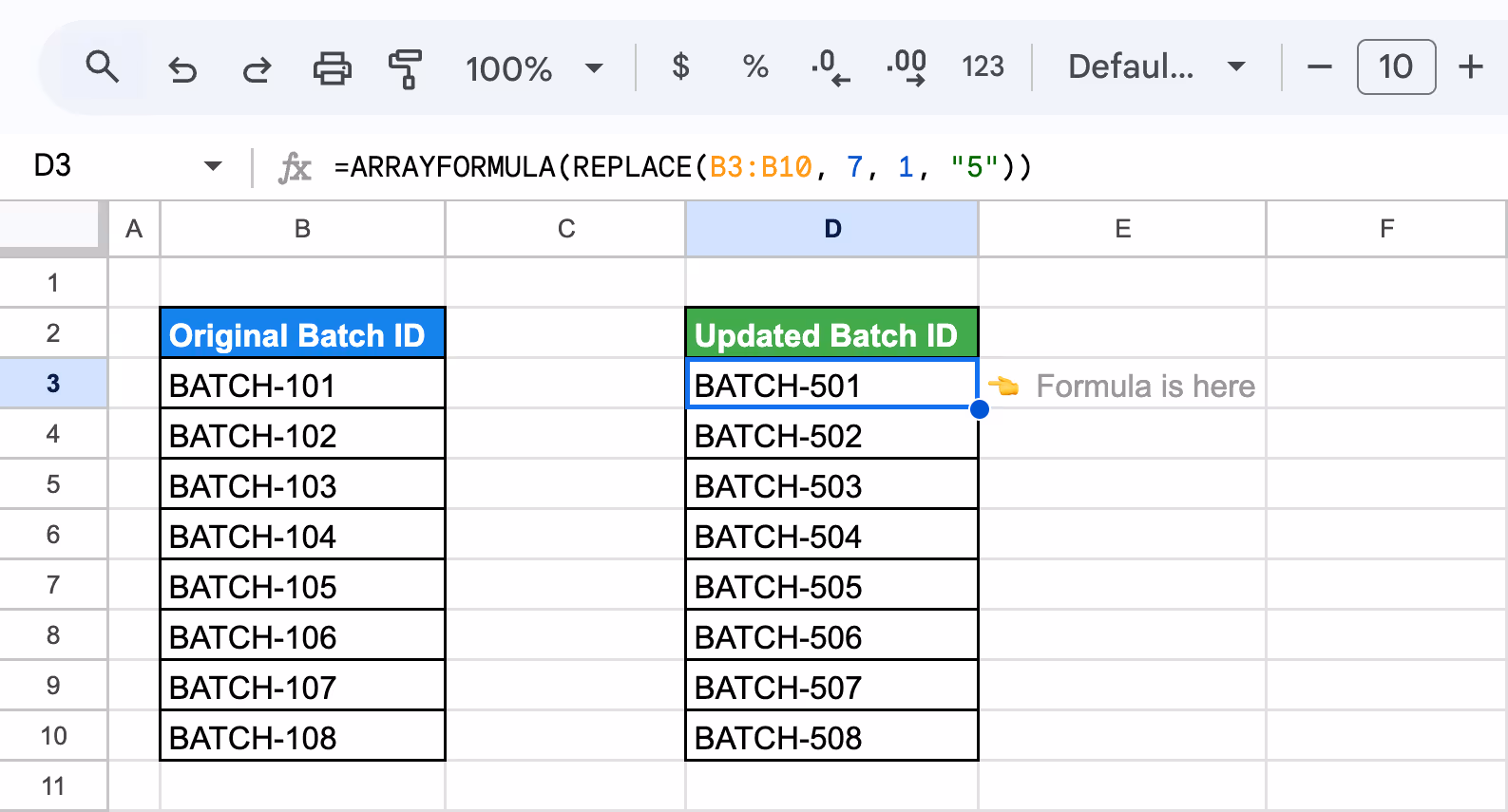
This method is useful when working with structured datasets that require bulk text modifications, ensuring accuracy and consistency while saving time.
Replace Text with Dynamic Values using FIND with REPLACE
In Google Sheets, combining the REPLACE function with FIND allows you to replace text dynamically based on its position in different cells. This is useful when the text to be modified appears at varying positions within different entries. Instead of manually identifying positions, FIND locates the exact position, and REPLACE updates the text accordingly.
Suppose you have a list of product codes where the letter "X" needs to be replaced with "Y", but its position varies in each code. Instead of manually specifying positions, FIND helps locate "X", and REPLACE updates it dynamically.
To achieve this, use the formula:
=REPLACE(B3, FIND("X", B3), 1, "Y")
Here’s the breakdown:
- B3: Refers to the original text or value in cell B3 that will be modified.
- FIND("X", B3): Locates the position of the letter "X" within the text in B3.
- 1: Specifies that only one character (the found "X") will be replaced.
- "Y": The new character that replaces "X" at the found position.

This method is efficient when modifying text dynamically across multiple entries, saving time and ensuring accuracy without manually identifying positions.
Conditional Text Replacement using REPLACE with IF Function
In Google Sheets, combining the REPLACE function with IF allows for conditional text replacement based on specific criteria. This is useful when you need to modify text only when certain conditions are met, ensuring more controlled updates. Instead of applying replacements to all values, the IF function helps determine when the change should occur.
Suppose you have a list of employee records where employees marked as "Inactive" need their ID suffix updated from "-TMP" to "-PERM" to indicate permanent removal, while others remain unchanged.
To achieve this, use the formula:
=IF(C3="Inactive", REPLACE(B3, 9, 3, "PERM"), B3)
Here’s the breakdown:
- C3: Refers to the employee status, which determines whether the replacement should occur.
- "Inactive": The condition being checked. If C3 contains "Inactive", the formula proceeds with the replacement.
- B3: Refers to the original employee ID that will be modified if the condition is met.
- 9: Specifies the starting position where the replacement begins (the 9th character in the text).
- 3: Indicates that three characters will be replaced.
- "PERM": The new text, replacing the existing three-character suffix ("TMP").
- B3 (in the ELSE condition): If the status is not "Inactive", the original employee ID remains unchanged.

This method ensures that only relevant records are updated, preventing unnecessary modifications and making conditional text replacement more efficient in large datasets.
Combine and Replace Text Strings using REPLACE with CONCATENATE
The REPLACE function can be combined with CONCATENATE in Google Sheets to join and modify text dynamically. This is useful for formatting structured data, updating references, or creating standardized codes while making targeted text replacements. By merging multiple text values and applying the REPLACE function, you can efficiently generate customized results.
Suppose you have a list of product categories and item numbers, and you need to generate a structured product code while replacing a specific character after merging the values.
To achieve this, use the formula:
=REPLACE(CONCATENATE(B3, "-", C3), 9, 1, "X")
Here’s the breakdown:
- B3: Refers to the first text value (e.g., a category or label) that will be combined.
- "-": Adds a hyphen as a separator between the two text values.
- C3: Refers to the second text value (e.g., an item number) that will be combined with B3.
- CONCATENATE(B3, "-", C3): Merges the values from B3 and C3 with a hyphen in between.
- 9: Specifies the starting position where the replacement should occur in the merged text.
- 1: Indicates that only one character will be replaced.
- "X": The new character that replaces the existing character at the specified position.

This approach is useful for structured data management, ensuring uniform product codes, and automating bulk text replacements efficiently.
Replace Characters and Convert Text to Lowercase using REPLACE with LOWER
Combining the REPLACE function with LOWER in Google Sheets allows users to modify text while ensuring all characters are converted to lowercase. This is useful for standardizing data formats, correcting text entries, and ensuring consistency across datasets. By applying the REPLACE formula first and then using LOWER, you can efficiently update and format text dynamically.
Suppose you have a list of product codes where a specific part of the code needs to be replaced, and the entire text must be converted to lowercase for consistency.
To achieve this, use the formula:
=LOWER(REPLACE(B3, 6, 3, "XYZ"))
Here’s the breakdown:
- B3: Refers to the original text or value in cell B3 that will be modified.
- 6: Specifies the starting position where the replacement should occur (the 6th character in the text).
- 3: Indicates that three characters will be replaced.
- "XYZ": The new text that replaces the existing three-character segment in B3.
- REPLACE(B3, 6, 3, "XYZ"): Modifies the text by replacing characters at the specified position.
- LOWER(...): Converts the entire updated text to lowercase.

This method ensures standardized formatting and text modifications, making data entry more uniform and reducing inconsistencies in large datasets.
Remove Extra Spaces with REPLACE and TRIM
When working with text data in Google Sheets, extra spaces can create formatting issues and inconsistencies. By combining REPLACE with TRIM, you can remove unwanted spaces while correcting specific parts of the text. This is particularly useful for cleaning up customer names, addresses, or other structured data where spacing errors may occur.
Suppose you have a list of addresses where extra spaces appear before and after commas, making the format inconsistent. You need to replace these spaces with a single comma, while also ensuring no unnecessary spaces remain.
To achieve this, use the formula:
=TRIM(REPLACE(B3, 12, 2, ","))
Here’s the breakdown:
- B3: Refers to the original text or value in cell B3 that will be modified.
- 12: Specifies the starting position where the replacement should occur (the 12th character in the text).
- 2: Indicates that two characters (extra spaces) will be replaced.
- ",": The new text that replaces the two spaces with a single comma.
- REPLACE(B3, 12, 2, ","): Modifies the text by removing extra spaces and inserting a properly formatted comma.
- TRIM(...): Ensures that any leading, trailing, or unnecessary spaces remaining in the text are removed.

This method is useful for standardizing address entries, improving data cleanliness, and ensuring proper formatting in reports and databases.
Count Characters with REPLACE and LEN
Using REPLACE with LEN in Google Sheets allows you to measure text length before and after making modifications. This is useful for tracking changes, ensuring consistency in structured data, and validating formatting adjustments. By comparing LEN before and after applying this REPLACE function, you can monitor how text modifications impact character counts.
Suppose you have a list of customer IDs, and you need to replace a specific portion of the ID while tracking the total number of characters before and after the modification.
To achieve this, use the formula:
=LEN(REPLACE(B3, 11, 2, "YYYY"))
Here’s the breakdown:
- B3: Refers to the original text or value in cell B3 that will be modified.
- 11: Specifies the starting position where the replacement should occur (the 11th character in the text).
- 2: Indicates that two characters will be replaced.
- "YYYY": The new text that replaces the existing two-character segment in B3.
- REPLACE(B3, 11, 2, "YYYY"): Modifies the text by replacing the characters at the specified position.
- LEN(...): Counts the total number of characters in the modified text after the replacement.

This method helps in tracking text modifications dynamically, ensuring text remains within specific length limits, and validating structured text formatting.
Common Issues with REPLACE Functions
Common issues with the REPLACE function include incorrect starting positions, unexpected results when working with numbers, and difficulty replacing multiple sections at once. Errors may also occur if the specified length exceeds the available characters. Ensuring accurate input values helps prevent unintended modifications.
Incorrect Starting Position Issues
⚠️ Error: The REPLACE function may not work as expected if the starting position is incorrect. If the position value is too low, it may replace unintended characters, while a value too high may result in no change. This often happens when working with varying text lengths or dynamic data.
✅ Solution: Always verify the position value before applying REPLACE. Use LEN() to check text length and ensure the position falls within valid limits. If working with dynamic content, functions like SEARCH() can help locate the correct starting point for replacements.
Mismatched Character Counts
⚠️ Error: The REPLACE function may not work as expected if the number of characters to be replaced does not match the intended portion of text. If the length is too short, only part of the text gets replaced, while an excessive length may remove unintended characters, altering the data structure.
✅ Solution: Double-check the length value to ensure it matches the intended characters. Use LEN() to determine the text length before replacing it. If working with variable-length text, functions like SEARCH() can help identify the exact portion that needs replacement.
Non-Text Data
⚠️ Error: The REPLACE function treats numbers as text, which can cause unexpected results. If used directly on a number, it may return a text-formatted result instead of a numeric value. This can lead to issues in calculations or sorting, especially when working with financial or statistical data.
✅ Solution: If replacing part of a number, wrap the REPLACE function with VALUE() to convert the result back into a number. Alternatively, store numbers as text if formatting is the primary concern. Always check data types to ensure the function behaves as expected.
Errors in Nested Formulas
⚠️ Error: Nesting the REPLACE function within other formulas can lead to errors if the referenced values are incorrect or dynamically changing. If a function within REPLACE returns an unexpected value (such as an empty cell or an error), the entire formula may break, leading to incorrect or missing outputs.
✅ Solution: Test each nested function separately before combining them. Use IFERROR() to handle potential errors and ensure valid inputs. When working with dynamic data, check for empty cells or unexpected results to maintain formula accuracy and prevent disruptions.
Case Sensitivity Issues
⚠️ Error: The REPLACE function does not differentiate between uppercase and lowercase letters—it simply replaces characters based on their position, regardless of case. This can lead to inconsistencies when modifying case-sensitive text, such as product codes, usernames, or formatted identifiers.
✅ Solution: If case sensitivity is important, consider using SEARCH() to locate specific text dynamically before applying the REPLACE. Alternatively, use LOWER(), UPPER(), or PROPER() to standardize text formatting before or after replacement to ensure consistency in case-sensitive data.
#REF!
⚠️ Error: A #REF! error occurs in the REPLACE function when it references an invalid cell or range. This can happen if a referenced cell has been deleted, the formula is incorrectly structured, or the position or length values exceed the available text, leading to an out-of-bounds reference.
✅ Solution: Check that all cell references in the formula are valid and ensure the position and length values do not exceed the text length. If a referenced cell has been deleted, update the formula with the correct reference. Using IFERROR() can help handle errors gracefully.
#NAME?
⚠️ Error: A #NAME? error in the REPLACE function usually occurs due to a typo in the function name, missing quotation marks around text values, or an undefined named range. If the function is misspelled or arguments are improperly formatted, Google Sheets cannot recognize the formula.
✅ Solution: Double-check that REPLACE is spelled correctly and ensure text values are enclosed in quotation marks. If using named ranges, verify that they are defined and correctly referenced. Properly formatting the formula prevents errors and ensures it functions as expected.
#ERROR!
⚠️ Error: A #ERROR! message in the REPLACE function indicates a formula parsing issue, often caused by incorrect syntax, missing arguments, or invalid data types. This can happen if the position or length values are non-numeric or if required parameters are left blank.
✅ Solution: Carefully check the formula’s syntax and ensure all required arguments are provided. Make sure position and length values are numeric and within the valid range. If working with dynamic data, use ISNUMBER() to verify numeric inputs before applying the REPLACE function to avoid parsing errors.
Best Practices and Tips for Using REPLACE Function
Using the REPLACE function efficiently involves understanding its structure, ensuring accurate modifications, and maintaining data consistency. Challenges may arise when handling different text formats, dynamic values, or unexpected errors. Proper planning and awareness of common issues help achieve smooth and reliable text updates in Google Sheets.
Ensure Position Numbers Are Within Text Length to Avoid Errors
To prevent errors when using the REPLACE function, ensure the position number falls within the text length. If the starting position is too high or the length value exceeds the available characters, the function may return unexpected results or errors. Use LEN() to check text length before applying the REPLACE and verify that position values align correctly to avoid modifying unintended parts of the text.
Convert Output to Numbers Using the VALUE Function
The REPLACE function returns a text string, even when modifying numbers. If numerical values are needed for calculations or sorting, use the VALUE function to convert the output back into a number. This ensures proper data formatting and prevents issues when working with numeric data in Google Sheets.
Use Appropriate Length Arguments to Prevent Replacing Excess Characters
If the length argument in the REPLACE function is greater than the number of characters remaining in the text from the specified position, it will replace all characters from that point to the end. To avoid unintended modifications, ensure the length value matches the exact portion of text that needs to be replaced.
Essential Google Sheets Functions for Smarter Data Search and Analysis
Google Sheets offers a range of advanced functions that go beyond basic search capabilities, making it easier to filter, analyze, and extract insights from large datasets. These functions help automate tasks, highlight specific patterns, and improve overall data accuracy and efficiency.
- VLOOKUP: Finds a value in the first column and returns a related value from another column—great for matching names with departments or roles.
- QUERY: Uses SQL-style syntax to filter, sort, and extract data based on custom conditions. Great for
- SEARCH: Returns the position of a specific substring within a text, helping identify whether certain keywords or values exist in a cell.
- SUM: Calculates the total of a range of numbers, useful for summing up figures like budgets, targets, or sales.
- AVERAGE: Computes the mean of a numeric range, ideal for evaluating performance indicators such as monthly averages or lead scores.
- COUNTA: Counts the number of non-blank cells in a range, making it effective for tracking entries and spotting missing data.
- HLOOKUP: Looks for a value in the top row of a dataset and returns the corresponding value from a specified row, best suited for horizontally structured data.
Simplify Your Data Visualization with OWOX: Reports, Charts & Pivots Extension
The REPLACE function is a great tool for modifying text, but what if you could automate even more? OWOX: Reports, Charts & Pivots Extension streamlines your workflow by generating dynamic reports, automating data updates, and integrating seamlessly with your spreadsheets.
Save time on tedious manual edits and focus on making data-driven decisions. Install the OWOX Reports Extension for Google Sheets today and experience a smarter way to manage your data!
FAQ

%202.png)

.avif)