Mastering the SUBSTITUTE Function in Google Sheets

Fixing or replacing text in large amounts of data can be tricky, but the SUBSTITUTE function in Google Sheets makes it much easier. This tool helps you quickly replace specific text within a cell, saving time and effort. Whether you’re cleaning up errors, standardizing text, or making updates, SUBSTITUTE is a simple way to keep your data tidy.

Anyone working with data students, professionals, or teams can benefit from this easy-to-use function. It’s flexible and takes care of repetitive tasks so you can focus on what matters most. Let’s go over how it works with some clear examples.

Overview of SUBSTITUTE Functions in Google Sheets 

The SUBSTITUTE function in Google Sheets is a powerful tool designed to replace specific text within a string with another. This makes it incredibly useful for tasks like correcting typos, standardizing text formats, or updating values without manually editing each cell. Whether you're dealing with product codes, names, or phone numbers, the SUBSTITUTE function helps streamline your work.

One of the key advantages of SUBSTITUTE is its flexibility. You can use it to replace all occurrences of a text string or target a specific instance by specifying which occurrence to replace. This is especially handy when you need precise control over your data updates.

Exploring the SUBSTITUTE Functions (With Syntax and Examples) 

Replacing specific text within a cell is simple and efficient with the SUBSTITUTE function in Google Sheets. This tool is ideal for cleaning, updating, and standardizing data quickly and accurately. Let’s dive into its syntax and practical examples.

The SUBSTITUTE function is perfect for correcting mistakes, modifying values, or standardizing formats, helping you save time and enhance data accuracy.

Syntax of SUBSTITUTE Function

=SUBSTITUTE(text_to_search, search_for, replace_with, [occurrence_number])

Let’s break down the parameters:

• text_to_search: The text or cell containing the string you want to modify.
• search_for: The specific text within the string that you want to replace.
• replace_with: The new text that will replace the specified text.
• occurrence_number (optional): The specific instance of the text to replace. If omitted, all occurrences are replaced.

By specifying the occurrence, you can target precise updates while keeping other parts of the text unchanged.

Example of SUBSTITUTE 

Let’s say you have a dataset where column D contains the reporting manager names, and you want to replace the last name "Carter" with "Johnson" for all entries.

Syntax:

=SUBSTITUTE("James Carter", "Carter", "Johnson")

Here:

• "James Carter": Refers to the original text or cell you want to modify.
• "Carter": Specifies the text to be replaced.
• "Johnson": Is the new text that will replace the specified text.

The formula replaces "Carter" with "Johnson," transforming the name into "James Johnson". The updated results appear in column F, as shown in the dataset.

Using SUBSTITUTE with a Cell Reference

In real datasets, you’ll often want to modify values directly from cells rather than typing static text into the formula. The SUBSTITUTE function also works perfectly with cell references, making it ideal for bulk edits.

Let’s say you want to replace the last name "Carter" with "Miller" in the reporting manager column (Column D). You can use the formula below:

Formula:

=SUBSTITUTE(D6, "Carter", "Miller")

Here’s what each part means:

• D6: Refers to the cell that contains the original manager name.
• "Carter": Is the text you want to replace.
• "Miller": Is the new text that will replace the specified word.

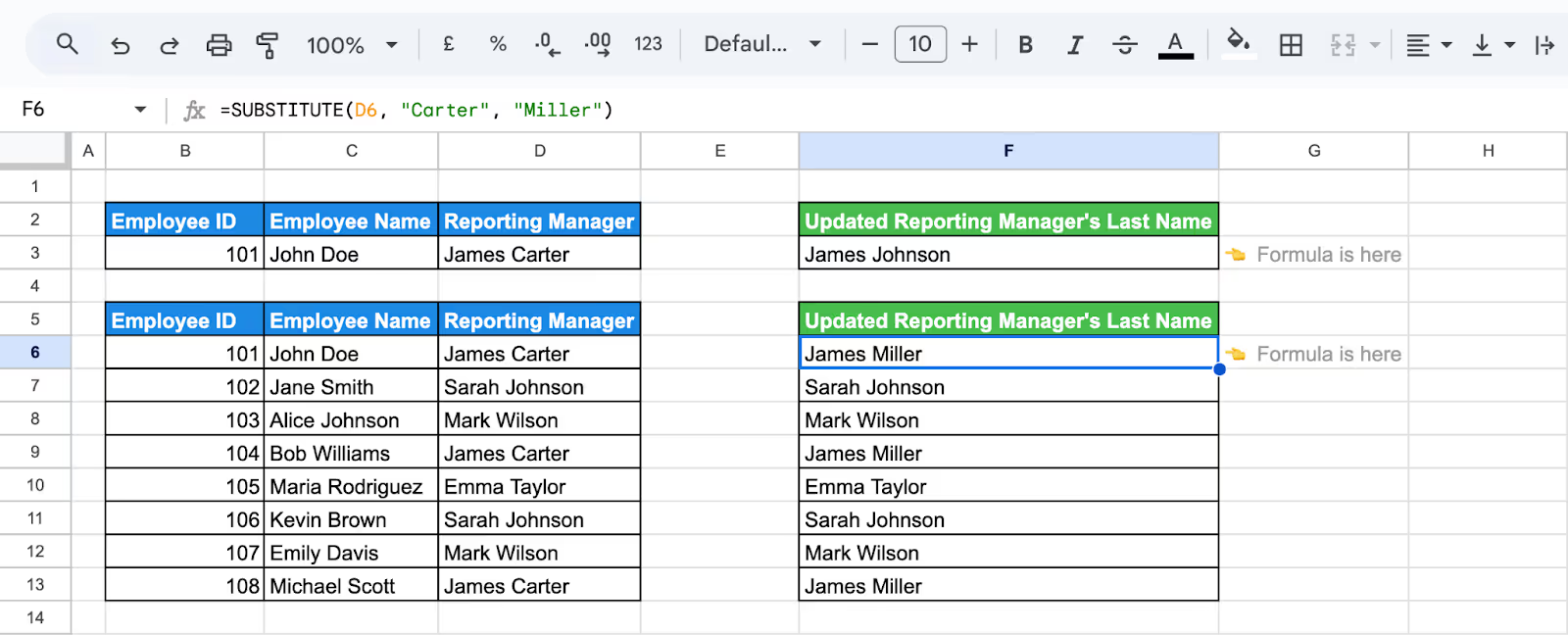
As shown in the updated dataset, every instance of "James Carter" becomes "James Miller" while other names remain unchanged. This approach is ideal for dynamic editing across rows using formulas.

Mastering Text Substitution in Google Sheets with the SUBSTITUTE Function with This Ready-to-use Template!

This downloadable file includes every example from the article, making it easy for you to practice and implement , Mastering Text Substitution in Google Sheets with the SUBSTITUTE Function in your own projects. Download, explore, and start mastering text substitution in Google Sheets with the SUBSTITUTE Function with ease!

Get your FREE template now!

Practical Examples of Using SUBSTITUTE Function in Google Sheets 

The SUBSTITUTE function in Google Sheets offers practical solutions for modifying text efficiently. From replacing specific characters to standardizing data formats, it helps streamline repetitive tasks, ensuring your dataset stays accurate and easy to work with. Let’s explore some practical examples.

Replace a Character in Text Using SUBSTITUTE 

The SUBSTITUTE function is a great tool for cleaning text data, such as removing unwanted characters like slashes ("/") and replacing them with spaces for better readability.

In the dataset, you have Employee IDs, Names and Departments with slashes in column C and want to clean them up by replacing the slashes with spaces.

Use the following formula in a new cell in column E:

=SUBSTITUTE(C3, "/", " ")

Here:

• C3: Refers to the cell containing the original employee name with slashes.
• "/": Specifies the character to be replaced.
• " ": Replaces the slash with a space.

This formula removes slashes and replaces them with spaces. The cleaned employee IDs, names with departments, are displayed in column E, as shown in the dataset.

Replace the First Occurrence in Text Using SUBSTITUTE

The SUBSTITUTE function in Google Sheets allows you to replace a specific occurrence of text. For example, you can target only the first slash ("/") in a text string and replace it with a space, leaving other slashes intact.

In the dataset, Employee IDs, Names with multiple slashes in column C, and you want to replace only the first slash with a space.

Use the following formula in a new cell in column E:

=SUBSTITUTE(C3, "/", " ", 1)

Here:

• C3: Refers to the cell containing the original text with slashes.
• "/": Specifies the character to be replaced.
• " ": Replaces the first slash with a space.
• 1: Indicates that only the first occurrence of the slash should be replaced.

This formula replaces only the first slash in each employee ID, name and department, and the updated IDs, names and departments are displayed in column E, as shown in the dataset.

Replace Text in a Single Cell Using SUBSTITUTE

The SUBSTITUTE function in Google Sheets is perfect for replacing specific text within a single cell. For instance, you can modify phrases in customer reviews to better align with updated language or tone.

In the dataset, the customer review in column D contains the phrase "truly excellent", which you want to replace with "outstanding".

Use the following formula in a new cell F3:

=SUBSTITUTE(D3, "truly excellent", "outstanding")

Here:

• D3: Refers to the cell containing the original review.
• "truly excellent": Specifies the text you want to replace.
• "outstanding": Is the new text that will replace the specified phrase.

This formula updates the phrase in the review, transforming it into a more polished version, as shown in the updated row in column F3.

Replace Specific Occurrences Using SUBSTITUTE

The SUBSTITUTE function in Google Sheets allows you to target and replace specific occurrences of a word or phrase within a cell. This is especially helpful when you want to update one instance of a repeated word while leaving others intact.

In the dataset, the customer reviews in column D contain the word "excellent" multiple times. If you want to replace only the second occurrence of "excellent" with "outstanding", use the following formula in cell F3:

Use the following formula:

=SUBSTITUTE(D3, "excellent", "outstanding", 2)

Here:

• D3: Refers to the cell containing the original review.
• "excellent": Specifies the word you want to replace.
• "outstanding": Is the new word that will replace the second occurrence.
• 2: Indicates that only the second occurrence of the word "excellent" will be replaced. 

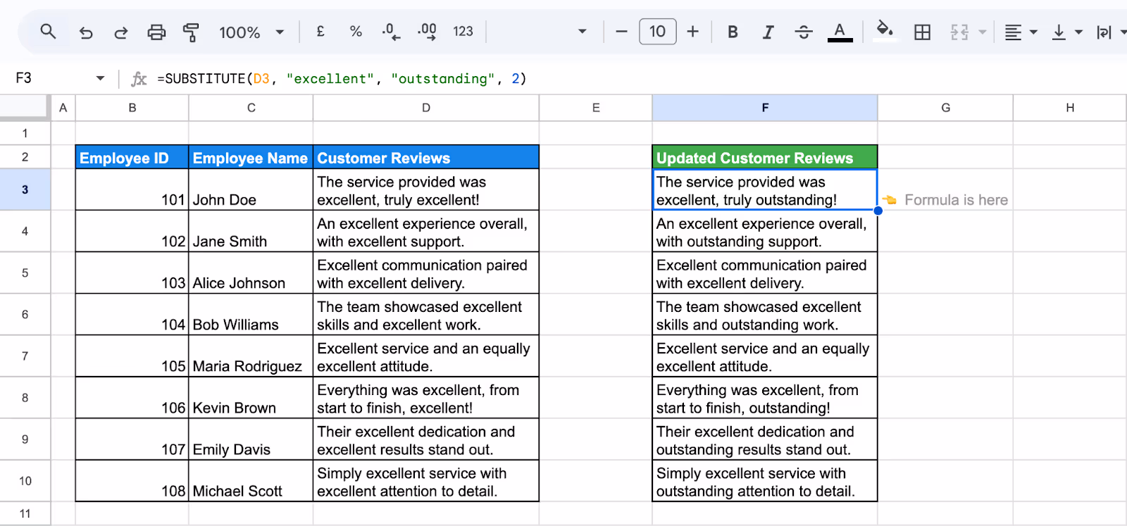
This formula updates only the second instance of the word "excellent" in the reviews, leaving the first instance unchanged. The results are displayed in column F3, as shown in the dataset.

Standardize Phone Number Formats with Nested SUBSTITUTE Functions

Phone numbers in datasets often appear in various formats, making them difficult to work with. Using nested SUBSTITUTE functions in Google Sheets, you can standardize phone number formats by removing unwanted characters such as parentheses ("(" and ")") and ensuring consistency.

In the dataset, the phone numbers in column C contain a mix of formats. To clean and standardize these numbers, removing parentheses and retaining only the digits with spaces or dashes, use the following formula in column E:

Use the following formula in a new cell in column E3:

=SUBSTITUTE(SUBSTITUTE(C3, "(", ""), ")", "")

Here:

• C3: Refers to the cell containing the original phone number.
• "(": The first SUBSTITUTE removes the opening parenthesis.
• ")": The second SUBSTITUTE removes the closing parenthesis.
• "": Replaces the unwanted characters with nothing (removes them).

This formula ensures all phone numbers are in a consistent format, free of parentheses, as shown in column E. Additional SUBSTITUTE functions can be added to remove other characters like dashes or dots if needed.

Using SUBSTITUTE with Other Google Sheet Functions 

By pairing SUBSTITUTE with functions like UPPER, LOWER, or ARRAYFORMULA, you can clean, standardize, and manipulate text effortlessly, even across large datasets. 

These combinations help you tackle complex scenarios, such as formatting text consistently or replacing values dynamically, all while saving time. Let’s dive into practical ways to use SUBSTITUTE with other functions.

Replace Text and Standardize Case Using SUBSTITUTE and UPPER Functions 

Combining the SUBSTITUTE and UPPER functions in Google Sheets allows you to replace specific text while converting everything to uppercase. This is especially useful for standardizing the format of reviews, names, or other text entries in a dataset.

In the dataset, the customer reviews in column D contain the word "excellent". To replace it with "Outstanding" and standardize all text to uppercase, use the following formula in column F3.

Here is the formula:

=SUBSTITUTE(UPPER(D3), "EXCELLENT", "OUTSTANDING")

Here:

• D3: Refers to the cell containing the original review.
• UPPER(D3): Converts the entire text in the cell to uppercase.
• "EXCELLENT": Specifies the text to replace (now in uppercase due to UPPER).
• "OUTSTANDING": Replaces the specified word with the new one.

This formula ensures all text is in uppercase while replacing every instance of "excellent" with "Outstanding", creating consistent and visually standardized reviews, as shown in cell F3.

Measure Text Length Using LEN and SUBSTITUTE Functions 

Combining the LEN and SUBSTITUTE functions in Google Sheets allows you to calculate the text length after replacing specific words or phrases. This is useful for analyzing text changes or standardizing data formatting.

Example:
In the dataset, the customer reviews in column D contain the word "excellent", which is replaced with "outstanding". To measure the length of the updated reviews, use the following formula in cell F3:

Here is the formula:

=LEN(SUBSTITUTE(D3, "excellent", "outstanding"))

Here:

• D3: Refers to the cell containing the original review.
• SUBSTITUTE(D3, "excellent", "outstanding"): Replaces the word "excellent" with "outstanding" in the text.
• LEN(...): Calculates the total length of the updated text string, including spaces and punctuation.

This formula replaces the specified word, updates the review, and measures the text length. The calculated length is displayed in cell F3, as shown in the dataset.

Substitute Multiple Values Using SUBSTITUTE with INDEX 

You can replace multiple values dynamically in Google Sheets by using SUBSTITUTE with INDEX. This method utilizes a reference table to find and replace text without requiring manual edits for each entry.

Let’s say you have Employee Names in column C that need to be replaced with their corresponding short forms from the Find (B13:B20) and Replace (C13:C20) columns.

Use the following formula in cell E3:

=SUBSTITUTE(SUBSTITUTE(SUBSTITUTE(C3, INDEX(B13:B20, 1), INDEX(C13:C20, 1)), INDEX(B13:B20, 2), INDEX(C13:C20, 2)), INDEX(B13:B20, 3), INDEX(C13:C20, 3))

Here:

• C3: Refers to the original Employee Name.
• INDEX(B13:B20, 1): Retrieves the first value to find from the "Find" column (John Doe).
• INDEX(C13:C20, 1): Retrieves the corresponding replacement value from the "Replace" column (JD).
• Second SUBSTITUTE (INDEX(B13:B20, 2), INDEX(C13:C20, 2)): Replaces the second value (Jane Smith → JS).
• Third SUBSTITUTE (INDEX(B13:B20, 3), INDEX(C13:C20, 3)): Replaces the third value (Alice Johnson → AJ).

This formula replaces employee names with their short forms dynamically, as shown in column E of the dataset.

Replacing Text Across Multiple Cells with SUBSTITUTE and ARRAYFORMULA 

In Google Sheets, the SUBSTITUTE function can be combined with ARRAYFORMULA to replace text across multiple cells at once. This is particularly useful for batch updates without manually editing each cell.

Example:
In the dataset, the Employee IDs in column B start with the prefix "OLD-". To replace it with "NEW-" across all rows, use the following formula in E3:

Use the following formula in column E3:

=ARRAYFORMULA(SUBSTITUTE(B3:B10, "OLD-", "NEW-"))

Here:

• B3:B10: Refers to the range of cells containing the original Employee IDs.
• "OLD-": Specifies the text you want to replace.
• "NEW-": Is the text that will replace the specified value.
• ARRAYFORMULA: Applies the SUBSTITUTE function across the entire range, ensuring all cells are updated simultaneously.

This formula dynamically updates all Employee IDs by replacing "OLD-" with "NEW-", and the results are displayed in column E.

Typical Issues with SUBSTITUTE Function in Google Sheets

The SUBSTITUTE function in Google Sheets is powerful but can lead to unexpected results if not used carefully. Common issues include case sensitivity, replacing unintended text, or failing to specify occurrences correctly. Understanding these challenges can help you avoid errors and ensure accurate data manipulation in your spreadsheets.

Mismatched Character Counts 

⚠️ Issue: When using SUBSTITUTE, replacing text with a string of significantly different length (shorter or longer) can result in formatting inconsistencies. For example, replacing "abc" with "123456" may misalign data or create uneven outputs.

✅ Solution: Check the character lengths of both the original and replacement strings using the LEN function to ensure they fit the intended format. If working with specific occurrences, ensure the correct occurrence number is targeted to avoid unexpected results.

Case Sensitivity Issues 

⚠️ Issue: The SUBSTITUTE function in Google Sheets is case-sensitive, meaning it distinguishes between uppercase and lowercase letters. For example, searching for "apple" will not replace "Apple" or "APPLE" in your data.

✅ Solution: To handle case sensitivity, use the LOWER or UPPER functions alongside SUBSTITUTE. Convert the text to a consistent case before performing the replacement. 

For example:
=SUBSTITUTE(LOWER(A1), "apple", "orange")

‍This ensures all instances of "apple," regardless of capitalization, are replaced.

Non-Existing Text 

⚠️ Issue: If the text you’re trying to replace with the SUBSTITUTE function doesn’t exist in the cell, Google Sheets won’t generate an error. Instead, it simply returns the original text unchanged.

✅ Solution: Use the SEARCH function to check if the target text exists in the cell before applying SUBSTITUTE. For example:

=IF(ISNUMBER(SEARCH("apple", A1)), SUBSTITUTE(A1, "apple", "orange"), A1)

This ensures replacements are made only if the target text is present, avoiding unnecessary operations.

#REF! 

⚠️ Error: The #REF! error occurs when a formula references a cell or range that has been deleted or is invalid. For example, using a formula like =A1+B1 will return #REF! if either A1 or B1 has been deleted.

✅ Solution: Review your formula to ensure all referenced cells or ranges exist. If the error is due to a deleted reference, recreate the missing range or update the formula to point to valid cells. For example, correct =A1+#REF! by replacing #REF! with the proper reference.

#NAME? 

⚠️ Error: The #NAME? error occurs when Google Sheets cannot recognize the text in a formula. This usually happens because of typos in function names, missing quotation marks around text strings, or referencing named ranges that haven't been defined.

✅ Solution: To resolve the #NAME? error, carefully review the formula. Ensure that function names are spelled correctly, text strings are enclosed in quotation marks (e.g., "Text"), and any named ranges used are properly defined. If the error persists, try re-entering the formula step-by-step to pinpoint the issue.

#ERROR!

⚠️ Error: The #ERROR! message indicates a formula parse error in Google Sheets. This happens when the formula is structured incorrectly, such as missing parentheses, improper use of operators, or incorrect syntax for a specific function.

✅ Solution: Carefully review the formula to ensure it follows the correct syntax and structure. For instance, check for missing parentheses, misplaced commas, or incorrect argument formatting. Re-entering the formula step-by-step can help identify and fix the issue efficiently.

Best Practices and Tips for Using SUBSTITUTE Function 

To get the most out of the SUBSTITUTE function in Google Sheets, it’s important to follow a few best practices. These tips will help you avoid common errors, streamline your workflows, and ensure accurate and efficient text replacements.

Using Backslash to Escape Special Characters 

When working with special characters or wildcards in Google Sheets, using a backslash (****) ensures they are treated as literal characters. For example, to replace "?", use the formula:

=SUBSTITUTE(A1, "\?", "replacement")

This method prevents characters like "?" or "*" from being misinterpreted as wildcards, ensuring accurate replacements.

Combine SUBSTITUTE function with other function 

The SUBSTITUTE function becomes more powerful when combined with other functions like TRIM, PROPER, LOWER, and UPPER. These combinations enable tasks like standardizing text, removing extra spaces, or formatting strings for better readability.

Example: To replace slashes while capitalizing words and removing spaces, use:

=PROPER(TRIM(SUBSTITUTE(A1, "/", " ")))

Essential Google Sheets Functions for Advanced Data Analysis

Google Sheets offers a powerful range of functions designed to simplify data analysis. These tools help manage and interpret complex datasets, uncover insights, and organize information efficiently, making detailed analysis more accessible and effective.

• VLOOKUP: Searches for a value in the first column of a range and retrieves a corresponding value from another column in the same row.
• HLOOKUP: Looks for a value in the first row of a range and returns a corresponding value from a specified row in the same column.
• CONCATENATE: Merges multiple text strings into one, simplifying the process of combining information from different cells.
• MATCH: Identifies the position of a specific value within a range, making it a key tool for lookups and comparisons.
• COUNTA: Counts all non-empty cells in a range, useful for tracking data entries and availability.
• XLOOKUP: A versatile replacement for VLOOKUP, providing advanced features like exact matches, reverse lookups, and error handling.

Streamline Your Data Visualization with OWOX Reports Extension for Google Sheets 

Streamline your data visualization process with the OWOX Reports Extension for Google Sheets. This powerful tool simplifies creating detailed reports, dynamic charts, and pivot tables, helping you easily organize and present data. It makes your data work smarter and is perfect for analyzing sales, marketing, or financial metrics.

Designed to enhance productivity, the extension automates repetitive tasks, minimizes errors, and ensures reporting accuracy. With advanced customization options, you can tailor charts and pivots to your needs, making data-driven insights clear and actionable. Save time and make confident decisions effortlessly.